
Lesson video
Narration is AI-generated. Video chapters, transcript and sources
Transcript
Transcript
UNIT-01 asks
Now and then a robot computes a dangerous action. Can we quietly fix it before it goes out? This episode, we build a safety filter. It sits between the policy and the motors. Safe actions pass. Dangerous ones get stopped.
Dangerous actions and the safety filter
Let's start with an example, the scene from this episode's notebook. A point robot on a flat plane. It has to go from the start to the goal. But right in front of it, there's a round obstacle. Its controller only cares about rushing to the goal. So it crashes straight in. This one that only rushes ahead, we call the nominal controller. It isn't bad. It just doesn't care about safety at all. Think how common this is. A learned policy is right almost all the time. But that one percent could cause an accident. You might ask, why not train a model that never makes mistakes? Because the world is too complex. You can't squeeze every danger into training. So think differently. Handle safety and intelligence separately. Let the clever part do the thinking. Let the reliable part catch the fall. This split has a big advantage. The policy can learn and explore boldly. Either way, there's a safety net underneath. So how does it work? Between the policy and the motors, add a filter. At every step, it asks one question. Is this action safe? If it's safe, let it through. If not, change it to the closest action that is safe. The smaller the change, the better. So there's no need to retrain the model! Just bend the action back into the safe zone at the last moment. Compare these two paths. The one that only rushes ahead runs into the obstacle. The one with the filter goes smoothly around.
Writing safety as a function
The key step is writing safety as a number. The distance to the obstacle, minus a safety radius. We call this number h. The paper only sets the convention: h at least zero counts as safe. Our choice of h has a nice property. It's positive when safe, negative when dangerous, and exactly zero on the boundary. The paper calls the region where h is at least zero the safe set. Put simply, being safe means staying inside this region forever. The paper gives an elegant condition. As long as every step satisfies one inequality, you can never leave the safe set. Let's stress the idea again. We don't change the task's goal. We just add one safety constraint on top of it. What does this inequality say? It says the safety margin can't fall too fast. The closer you get to the boundary, the more you hold back. For our point robot, this condition happens to be linear in the action. Linear means easy to solve. That matters a lot. So the safety filter becomes a small optimisation problem. The goal is to stay as close as possible to the nominal action. The constraint is that inequality. This kind of problem has a name, a quadratic program. It's tiny, with just one constraint. It's solved in the blink of an eye. By the way, where does this function h come from? You can write it by hand, or learn it from data. A learned one is called a neural barrier function. One more thing: safety here is relative to the model. The model thinking it's safe isn't enough. Only if the model is accurate is the robot really safe. So safety isn't about praying! It's solving one small problem, for real, at every step.
Into the fastest loop
How fast can a small problem like this be solved? On a palm-sized board, one paper measured a different quadratic-program controller. On average, about zero point four milliseconds. That order of magnitude is fast enough. We recommend putting the safety filter on the fastest loop. One robot-arm paper says real-time control needs a thousand times a second. Why does it have to be this fast? Because danger often appears suddenly. One step late, and it's too late to stop. It's also gentle. Far from the obstacle, it barely touches your action. Only near the boundary does it gently bend it back. This is called minimally invasive. If it can stay out, it stays out. It steps in only when it must. Another plus, it's explainable. Why it changed an action, you can see line by line. For safety, that's crucial. So a good safety layer is one you don't even notice most of the time! Let's be clear about its place. It doesn't decide for the model. It steps in only at the instant of crossing the line. The rest of the time, the model is in charge. It can handle several rules too. Don't hit the wall, don't speed, don't tip over. Write them all as inequalities, and put them in the same problem. Several rules can clash. You want to avoid the obstacle, but not slam the brakes. The problem finds a compromise action for you. But don't treat it as insurance for everything. All these guarantees rest on one assumption. The model has to be accurate enough. The distance, the dynamics, the gradient, all have to be accurate. If even one is off, the safety guarantee gets weaker. There are harder cases. If you control acceleration, not velocity, the relative degree is higher. You need higher-order methods. Actuators also saturate. A motor's strength always has a limit. Sometimes it wants to stop the robot, and really can't. So be honest about its limits. It can block a lot of accidents. But it is not a guarantee of absolute safety. Open this episode's notebook and follow along. First turn the filter off, and watch it crash. Then turn it on, and watch it go smoothly around. Now look at the curve of h. Without the filter, it drops below the zero line. With the filter, it always stays above it. You can also tune one parameter, alpha. It decides how decisive the filter is. Larger is more agile, smaller more cautious. Watch that line stay firmly above zero with your own eyes. That's what safe looks like! Let's recap, three points. One, write safety as h. Safe means the margin h never drops below zero. Two, the filter is a small quadratic program, minimally invasive. Three, it has to sit on the fastest loop, and the model has to be accurate. A safety filter doesn't make a robot smarter. It only promises one thing. However rushed, it never crosses that line! But how do we know this stuff really works? Next time, we talk about evaluation. See you next time!
Evidence and sources
Practice and self-check
- Interactive quiz5 questions, explained as you answer
- One-page summaryprintable; opens in a new tab
- Download the notebookszip in Chinese, English and Japanese; run in Jupyter or upload to Colab
The quiz is public and explains each answer as you go; answers to the guide's exercises are for signed-in members.
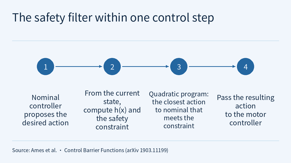
The video for episode 2.7 is about the safety filter: it sits between the policy and the motors, checks the action once per step, passes it if it is safe, and otherwise changes it to the closest action that is safe. The video makes three points. Write safety as a function h, so that the safe set is h(x) ≥ 0; if one inequality holds at every step, the safe set is forward invariant. The safety filter is a very small quadratic program that finds the action closest to the nominal one that still meets the safety constraint, which is what minimally invasive means. It has to sit on the fastest loop, and every guarantee assumes the model is accurate enough; higher relative degree and actuator saturation both weaken it. The three number cards in the video come from two public papers. Ames et al.’s survey Control Barrier Functions: Theory and Applications (arXiv 1903.11199) sets the convention that the region where h ≥ 0 is the safe set; the same paper reports, in its Segway experiment, an average computation time of 0.4 ms for the CLF-QP on a BeagleBone Black board; and the multipanda_ros2 paper (arXiv 2602.02269) says that sustaining a 1 kHz control frequency is a necessity for its real-time control and a minimum frequency required by safety standards. This page is the reading and exercises for the episode. It does not repeat the transcript. Instead it does three things the video only touches on: it reads Ames et al.’s definitions of the safe set, forward invariance and the control barrier function, to pin down what the video’s “one inequality” actually is and why it is linear in the action; it works one step of safety filtering through by hand for a hypothetical point robot; and it works out which loop the filter belongs on, how much of the safety margin is used up between two checks, and which assumptions, once broken, weaken the guarantee. One rule runs through the whole page: a CBF guarantee is relative to the model, and a computation time or a frequency belongs only to the system that measured or proposed it.
The video, transcript and sources for this lesson are at the top of this page; the season plan is in the course outline. The previous lesson, Physical AI Lab 2.6: To the Edge — Working Out the Control-Rate Ceiling from a Latency Log, Telling Whether Quantization Saves Size or Time, Then Sizing an Action Chunk, ended by asking: what if the model computes a dangerous action, who stops it? This lesson answers. The original 1 kHz sentence from multipanda_ros2, the command rates of the robots in that paper’s Table I, and “the rate ceiling is the reciprocal of one cycle’s latency” were covered in 2.6; turning rates into periods was worked through in Physical AI Lab 1.2: PID and Control Rate — Computing the Three Terms by Hand, Then Turning Rates into Periods; why a simulation model and a real robot disagree was covered in Physical AI Lab 2.5: Sim2real with Domain Randomization and System Identification — Putting Two Papers’ Numbers Back in Their Setups, Then Working Out Friction by Hand from One Push of a Cup. This lesson does not repeat them. It covers the CBF itself and the calculations needed to put one into a loop. The next episode, 2.8, is about reproducible evaluation with repeated trials and confidence intervals.
The public quiz’s 5 questions come with full explanations. Signed-in readers can do three exercises: work out the safety filter by hand at four states of a fictional point robot and see which corrections disappear when the parameter a changes; choose the loop for the filter on a fictional mobile base and work out, from the period, latency and range error, how much margin the safety radius must keep; and review a fictional safety plan, putting each sentence back into the two papers’ original conditions and checking the value of a against the loop period. Each comes with a step-by-step solution, common mistakes and a 20-point rubric.
1. What each paper says
Ames et al., Control Barrier Functions: Theory and Applications (arXiv 1903.11199; this lesson reads HTML v1). The abstract describes the paper as an introduction and overview of recent work on control barrier functions and their use to verify and enforce safety properties in optimization-based safety-critical controllers. Under this course’s levels it is R. The “h ≥ 0” number card in the video corresponds to a sentence in the introduction:
Dually, invariance can be seen as an example of a safety property in the sense that any trajectory starting inside an invariant set will never reach the complement of the set, describing the locus where bad things happen.
Section II of the paper turns this sentence into definitions:
- Safe set. Take a continuously differentiable function h; the safe set 𝒞 is all states with h(x) ≥ 0, its boundary is h(x) = 0, and its interior is h(x) > 0 (equation 5). The paper only sets this convention; “distance to the obstacle minus a safety radius” in the video is the h this course chose.
- Forward invariance and safety. Definition 1: 𝒞 is forward invariant if, starting from any point in 𝒞, the solution of the closed-loop system stays in 𝒞 for its whole interval of existence; the system is safe with respect to 𝒞 if 𝒞 is forward invariant. The “system” here is the closed-loop model the paper writes down,
ẋ = f(x) + g(x)k(x), assumed to be locally Lipschitz. - Control barrier function. The paper assumes a control-affine system,
ẋ = f(x) + g(x)u. Definition 2: h is a control barrier function if there is an extended class 𝒦∞ function α (strictly increasing, with α(0) = 0) such thatsup_u [L_f h(x) + L_g h(x) u] ≥ −α(h(x))for all x. The expression in brackets is exactly the rate of change ḣ of h along the system. - Why “minimally invasive”. The introduction says that the condition “there exists u such that ḣ(x, u) ≥ −α(h(x))” is necessary and sufficient (for compact sets) and so minimally restrictive; and because it holds over the whole of 𝒞, it gives a way to synthesize safe controllers through optimization-based control methods that modify the desired controller in a minimally invasive fashion.
- The difficulties the paper itself lists. The overview says that Section III treats systems with actuation constraints and Section IV constraints with higher relative degree. The video’s closing “actuator saturation” and “higher relative degree” correspond to those two sections; this lesson did not read their methods.
The “0.4 milliseconds” number card in the video comes from the Segway experiment in Section V of the paper. The original sentence is:
the CLF-QP was solved onboard the hardware on a BeagleBone Black with an average computation time of 0.4 ms
Read it together with its context:
- What safe means. The Segway’s safety constraint is staying upright, keeping the pendulum angle ϕ within [−π/12, π/12] rad; the nominal controller is a standard PD controller that tracks a desired signal.
- h is not two hand-written bounds. The paper says one might be tempted to use two simple control barrier functions on the upper and lower angle bounds; they could be implemented via a CBF-QP, but they would not enforce all of the additional constraints necessary for experimental implementation. So the authors used the Hamilton-Jacobi method, performing a reachability analysis over a 75×75×75 grid of the state space to find the safe set that satisfies those constraints, and then used polynomial regression to obtain an analytic expression that can be used in the safety filter.
- What 0.4 ms is. It is an average computation time; the object solved in that sentence is the CLF-QP, and the resulting signal u_act is passed to the motor controller. The same paragraph describes “with the ASIF” as “the CLF-QP active”; it does not time the CBF part separately, and it gives no worst case. The video cites it as “a different quadratic-program controller”, as an order-of-magnitude reference only, not as a measurement of this episode’s CBF filter.
- What the paper reports. The desired pendulum angle was a sinusoid with an amplitude exceeding π/12; the authors ran one experiment without and one with the ASIF and report that the system remains safe only when the safety filter implementing the CBF is active; when a kick was added as a disturbance, the system stayed upright with CBFs and failed without them. These are author-reported results; this site has not reproduced them.
multipanda_ros2 (Škerlj et al., arXiv 2602.02269; the page notes publication at ICRA 2026; level R). The “1 kHz” number card in the video corresponds to a sentence in the abstract:
A central focus of this work is sustaining a 1kHz control frequency, a necessity for real-time control and a minimum frequency required by safety standards.
2.6 has already put this sentence back into its torque-control framework. Only two statements in Section II of the paper matter for this lesson: safety standards such as ISO 10218 specify 1 kHz measurement frequencies for collision detection; and cobots often use cascaded architectures, where an outer loop generates task-level commands and inner loops regulate motor torques or velocities, improving precision and disturbance rejection while retaining fast safety responses. The paper does not discuss control barrier functions; “put the filter on the fastest loop” is this course’s design advice.
| Number in the video | From | Conditions in the original | What the original does not say | Level |
|---|---|---|---|---|
| h ≥ 0 | Ames et al., introduction and Section II | The safe set is the states with h ≥ 0; safety means the safe set is forward invariant for the closed-loop model | It does not prescribe how to choose h; “distance minus safety radius” is this course’s choice | R |
| 0.4 milliseconds | Ames et al., Section V Segway experiment | The CLF-QP, solved on a BeagleBone Black; average computation time | Not a measurement of this episode’s filter; no worst case; says nothing about other hardware or other problems | R (author-reported) |
| 1 kHz | multipanda_ros2, abstract and Section II | That framework’s real-time torque control; the paper says ISO 10218 and others specify a 1 kHz measurement frequency for collision detection | Nothing about CBFs, and no frequency requirement for a safety filter; this lesson did not consult the text of ISO 10218 | R (author statement) |
Sign in to keep reading: the rest of this lesson, its self-check questions and the answers.
Limitations
- Ames et al. (arXiv 1903.11199, HTML v1) is level R and a survey. This lesson read the abstract, the introduction, Section II up to Remark 3, and the Segway paragraphs of Section V; it did not read the methods in Sections III and IV. The closed-form solution in section 2, the bound in section 3 and the derivations in section 4 were derived in this lesson from the paper’s definitions; the paper does not state them.
- 0.4 ms is an author-reported average computation time, and the original sentence names the CLF-QP as the object solved; the paragraphs read give no worst case and do not spell out ASIF. The video cites it as “a different quadratic-program controller”, as an order-of-magnitude reference only.
- multipanda_ros2 (arXiv 2602.02269) is level R, and the page notes publication at ICRA 2026; the 1 kHz and the statement about ISO 10218 are the authors’ statements, and this lesson did not consult the text of ISO 10218. The paper does not discuss control barrier functions.
- The following are this lesson’s choices, advice or inferences: h = distance − safety radius; α(h) = a·h; the velocity-controlled point-robot model; the bound on the fall between two checks; the first-order approximation a·T ≤ 1; advice such as “put the filter on the fastest loop that sends u”, “check every step while executing a chunk” and “define the behaviour on infeasibility or overrun”; and the observation that a robot heading straight at the centre only slows and never goes around.
- The obstacles, radii, positions, speeds, values of a, rates, latencies, range errors, deceleration, mobile base, planner V and team Z in sections 2 to 5 are fictional; 0.30, 0.28, 0.032 m, 0.052 m, 1.5 and so on hold only under these assumptions.
- This lesson did not run the episode’s Notebook and did not check its start and goal, parameters or saved results.
- Calculations on paper and simulation results are not hardware safety validation; trials on a real robot need their own safety preparation and an independent safety measure unrelated to the filter.
Links
- Physical AI Lab: a physical AI course where every number can be checked (course outline)
- Physical AI Lab 2.6: To the Edge — Working Out the Control-Rate Ceiling from a Latency Log, Telling Whether Quantization Saves Size or Time, Then Sizing an Action Chunk
- Physical AI Lab 2.5: Sim2real with Domain Randomization and System Identification — Putting Two Papers’ Numbers Back in Their Setups, Then Working Out Friction by Hand from One Push of a Cup
- Physical AI Lab 1.2: PID and Control Rate — Computing the Three Terms by Hand, Then Turning Rates into Periods
- Ames et al.: Control Barrier Functions: Theory and Applications (arXiv 1903.11199, HTML v1)
- Bridging the Sim-to-Real Gap with multipanda_ros2: A Real-Time ROS 2 Framework for Multimanual Systems (arXiv 2602.02269)