Lesson video
Narration is AI-generated. Video chapters, transcript and sources
Transcript
Transcript
UNIT-01 asks
Stand a chopstick up on your palm. Why does your hand have to keep moving to stop it falling? Last time we worked out the joint angles. This time it's control: how a robot makes what actually happens steadily catch up with the target. Think of cruise control. Going uphill, the speed drops, so it gives more gas and pushes the speed back up. That's a controller at work.
Closed loop: measure, compare, act
At the heart of control is a loop. First measure where you are now, then compare it with the target. How far off you are is the error. Then this error decides how hard the motor pushes. Far off, it chases hard. Close, it eases off gently. If it doesn't measure, and just follows moves programmed in advance, that's open loop. If something disturbs it along the way, it doesn't know, and doesn't correct. This loop of measuring and correcting, going round again and again, is called closed-loop control. It's what physical AI relies on. Controllers like this, measuring and correcting, have a classic recipe called PID. One study estimates that nine in ten controllers in industry are of this kind.
Three flavours of PID: proportional, integral, derivative
First P, proportional. The bigger the error, the harder it pushes. The smaller the error, the gentler. It does the heavy lifting. Roughly speaking, an inverter air conditioner's thermostat works a bit like proportional control. The further from the set temperature, the harder the air conditioner runs. Close to it, it slows down on its own. But with P alone, it easily overshoots. It shoots past, gets pulled back, and swings back and forth, taking ages to settle. Then add I, integral. It adds up past errors, bit by bit. However small the error, it won't let it go. It's the cure for always being just a little bit off. Once enough has built up, it fills in that little tail. This is called steady-state error. Finally, D, derivative. It watches how fast the error is changing. Nearing the target, it eases off early. D is like a brake. It adds damping to the system and holds down the shaking. The faster things change, the harder it holds. P does the heavy lifting, I makes up the last small gap, D hits the brakes. Tune all three together, and it's fast and steady. Tune them badly, and it shakes, or it drifts. So PID isn't three switches. It's three tempers that have to be balanced!
Control rate: how fast the loop turns
Even with PID tuned well, there's one more thing. How many times a second can this loop go round? That's called the control rate. Some things are unstable by nature, like a pole standing upright. Let go, and it falls. You have to measure and correct without a moment's pause. If the loop turns too slowly, things go wrong. By the time you react, the pole has already fallen. It's like driving with your eyes shut, opening them every few seconds. The faster it turns, the sooner it corrects, and the steadier it is. A gust of wind, a shaky hand, and before it can drift off, it's already corrected. Take one force-controlled robot arm. Its maker says its low-level control runs a thousand times a second. That's one kilohertz, measuring and correcting at every tick. If the rate can't keep up, even the best-tuned PID is no use! Open this episode's page. On screen there's an upside-down pole, held up entirely by a controller. Without it, it falls. First drag P up and watch it swing back and forth. Add a little D, and the shaking dies down. The pole slowly steadies. Then add the integral term to fill in that tail that's always a little off. Last, lower the control rate, and watch the pole wobble and fall. A note: there's no universal formula for tuning a P-I-D controller. Mostly it's found by trying, bit by bit. Tweak it, watch the response, tweak again. PID is simple and handy, but it doesn't understand your machine. For very complex systems whose parts interfere with each other, you need a smarter controller. Let's recap, three points. One, the closed loop: measure, compare the error, then act. Two, the three flavours of P-I-D: P pushes, then I fills the gap, D hits the brakes. Three, the control rate must be high enough. If the loop turns slowly, even the best P-I-D controller cannot hold steady. So a standing chopstick needs constant motion, because it's always measuring, correcting, and chasing! But to correct mistakes, you first have to measure accurately. What does a robot use to sense the world? See you next time!
Evidence and sources
Practice and self-check
- Interactive quiz5 questions, explained as you answer
- Browser labno install: drag and tune it yourself
- One-page summaryprintable; opens in a new tab
The quiz is public and explains each answer as you go; answers to the guide's exercises are for signed-in members.
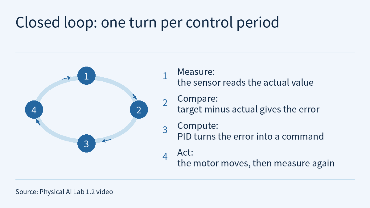
The episode 1.2 video uses “a chopstick standing on your palm” to teach three things. Control is a loop that keeps turning: measure what actually happens, compare it with the target to get the error, then act on the error. The three PID terms each have a job: P does the heavy lifting, I fills in the steady-state error, D works like a brake. How many times a second the loop goes round is the control rate, and if it turns too slowly, even the best-tuned PID cannot hold steady. The video cites two pieces of evidence: a review chapter relays that about nine in ten industrial controllers are of the PID kind, and the maker of one force-controlled robot arm, the Franka Research 3, states that its motion control runs at 1 kHz. This page is the episode’s reading and exercises. Rather than repeat the transcript, it first sets out the scope of each piece of evidence, then uses hypothetical numbers to compute three steps of PID output by hand and watch the integral term fill in the “little tail”, and finally turns control rates into periods to estimate how far a hypothetical pole drifts between two corrections. One rule runs throughout: a number holds only for the source that gives it and the kind of system it describes.
The video, transcript and sources for this lesson are above on this page; the whole season is in the course outline. The previous lesson, Physical AI Lab 1.1: Coordinate Frames and Kinematics — Working Out by Hand How a Two-Link Arm Reaches the Cup, ended by asking: the joint angles are worked out, so how does the motor turn there steadily? This lesson picks up that question. Physical AI Lab 0.3: See, Think, Act — Putting Each Rate Back in Its Own System already set the FCI’s 1 kHz on a different product page (Franka TMR) apart from two other rates; this lesson cites the stated figure on the Franka Research 3 product page, does not repeat that table and uses the figure only to practise converting rates into periods.
The five public quiz questions come with full explanations. Signed-in readers get three exercises: work through a fictional PID log that contains a disturbance, and catch a controller that was moved to a new rate without updating dt; compute rise time, overshoot, settling time and steady-state error from two fictional response records, using the review chapter’s definitions; and review a fictional control-rate memo with this lesson’s pole model. Each comes with a worked solution, common mistakes and a 20-point rubric.
1. Two pieces of evidence, each with its own scope
“Nine in ten” is relayed by a review chapter. The figure in the video comes from IntechOpen’s Introductory Chapter: PID-Based Industrial Process Control, by Mohammad Shamsuzzoha (Billington Process Technology, Norway) and G. Lloyds Raja (National Institute of Technology Patna, India). The original sentence is:
Another study states that about 90% industrial controllers are of PID type [ 2 ] to meet the requirement.
Four things to note when reading it:
- It is relayed. The “another study” in the sentence is reference [2], O’Dwyer’s Handbook of PI and PID Controller Tuning Rules (2009). The chapter does not say how the share was counted, and this lesson has not consulted the handbook. Under the course’s grading it is cited at level R.
- The context is process control. The chapter opens by stating that a PID controller is used at the regulatory level of industrial control to regulate process variables such as temperature, pressure and flow. “Nine in ten” refers to industrial controllers of this kind, not robot joints; the source gives no figure for robots.
- The same paragraph has another number from another source. The sentence just before it says another study concluded that the industrial preference for PID, advanced control and model predictive control is in the ratio 100:10:1. That is reference [1], a questionnaire survey of chemical process control in Japan by Kano and Ogawa (2010). The two numbers come from two sources that counted different things and cannot be merged into one conclusion.
- It is a usage share, not a capability. The chapter also lists limits of PID schemes: a unity-feedback structure is not suitable for plants with large time delays and disturbances, and many of the strategies it discusses apply only to single-input single-output systems and need careful redesign to extend to multi-input multi-output (MIMO) systems. The video ends by saying that complex systems whose parts interfere with each other need a smarter controller; the chapter’s wording can serve as the matching literature background.
“1 kHz” is one product’s maker-stated figure. The original sentence on the Franka Research 3 product page is:
High-frequency (1 kHz) motion control with a low-level, high-quality sensor data interface, ideal for motion control research and the development of highly specific behaviors, unachievable with most robots.
The same page says this rate belongs to the Franka Control Interface (FCI): researchers can run their own control algorithms at 1 kHz on external real-time capable PCs; through libfranka, the open-source C++ interface, they can send real-time control values at 1 kHz through 5 interfaces (joint torque with gravity and friction compensation, joint position, joint velocity, Cartesian pose, Cartesian velocity), and at the same time receive 1 kHz measurements such as joint position, velocity and torque sensor signals. What this supports:
- 1 kHz is the stated rate of this product’s external control interface. It is the maker’s own description (level O), not a measurement by this site. The page does not give the rates of any lower-level loops inside the arm.
- “Unachievable with most robots” is the maker’s own comparison; the page gives no data for it.
- It shows that this arm can exchange commands and measurements once every 1 ms. It does not show that PID has to run at 1 kHz, nor anything about other arms’ rates. How fast a loop needs to be depends on how fast the controlled object itself changes; section 4 works this through with hypothetical numbers.
Sign in to keep reading: the rest of this lesson, its self-check questions and the answers.
Limitations
- IntechOpen’s Introductory Chapter: PID-Based Industrial Process Control is cited at level R. “About 90%” is its relay of O’Dwyer’s handbook [2], and “100:10:1” its relay of Kano and Ogawa’s survey of chemical process control in Japan [1]; this lesson has not consulted either original source and does not know how they were counted. Both numbers are set in industrial process control.
- Franka Research 3’s 1 kHz motion control and the descriptions of FCI and libfranka all come from the maker’s product page, the maker’s own description (level O), not independently verified by this site; “unachievable with most robots” is the maker’s own comparison.
- The target angle, measurement readings, gains, pole lengths and initial tilt in sections 2 to 4 are assumptions for the exercises, not parameters of the video’s lab page or of any real system. The formula in section 2 is one way of writing a discrete PID, and “D is 0 at the first step” is this example’s convention.
- Section 4’s model reduces the pole to a point mass at the top of a fixed pivot, uses only the small-angle linear approximation, and assumes no correction at all between measurements. It ignores the command the controller holds during each period, delay, noise and motor capability, and it is not a stability analysis.
- The record sheet in section 5 is a teaching suggestion. This page has not checked how the video’s lab page is implemented.
- In section 6, the joint, gains, readings, porting case, records A–C, the teammate’s remark, team W, the two poles, the 20 Hz camera, the 200 Hz loop, the 30 ms delay and memo sentences M1–M3 are all invented for practice; results such as −0.08, 1.90, 0.4 s, 0.6 s, 25%, 1.5%, about 1.063°, about 1.57° and about 1.13° hold only under these assumptions. Task 1’s statement about oscillation is an inference from the division of labour among the PID terms, not a simulation result; task 1’s transfer exercise shows only the arithmetic of this lesson’s formula and says nothing about how real implementations handle noise.
- The definitions of rise time and settling time come from the review chapter; the overshoot percentage, the rules for reading sample points and task 3’s folding of delay into the interval are this lesson’s conventions. The suggested rewrite in task 3 is a teaching suggestion, not a conclusion from any source; paper calculations, the lab page and simulations are not hardware safety validation.
Links
- Physical AI Lab: a physical AI course where every number can be checked (course outline)
- Physical AI Lab 1.1: Coordinate Frames and Kinematics — Working Out by Hand How a Two-Link Arm Reaches the Cup
- Physical AI Lab 0.3: See, Think, Act — Putting Each Rate Back in Its Own System
- IntechOpen: Introductory Chapter: PID-Based Industrial Process Control
- Franka Robotics: Franka Research 3 product page