The preprint Online Hamilton–Jacobi Reachability Onboard the Robot Control Loop (arXiv 2611.04096, 2026-11-03, by Kevin Weekly of Mirror AI and Alexandre M. Bayen of UC Berkeley) does not propose a new numerical scheme. It writes the standard level-set solver of Hamilton–Jacobi (HJ) reachability analysis (WENO5 + TVD-RK3 + Lax–Friedrichs) as CUDA kernels, so that the backward reachable tube (BRT) can be recomputed at the pace of a robot’s control loop instead of once, offline, before a mission. The authors report that in FP32 on one RTX 4000 Ada workstation GPU a single solve of the classic 3D Air3D case takes 8.91 ms, about 112 Hz, and that on a Jetson AGX Thor it runs at 66 Hz at N = 41. These numbers have to be read together with grid resolution, precision and state dimension: the paper covers only 2D to 4D, and its safety guarantee holds only relative to the dynamics and disturbance model written down. All numbers below are author-reported [R]; this site has not reproduced them.
What a backward reachable tube is, and why compute it online
The paper uses the definition of Mitchell, Bayen and Tomlin. A system ẋ = f(x, u, d) has a control u and a disturbance d, and a failure set is described by a signed-distance function ℓ (ℓ(x) ≤ 0 means failure). The time-T backward reachable tube is the set of initial states from which, whatever the control does, the worst-case disturbance can push the system into the failure set within T. It equals the zero sublevel set {x : V(t, x) ≤ 0} of a value function V; V satisfies the Hamilton–Jacobi–Isaacs (HJI) partial differential equation with Hamiltonian max_u min_d pᵀf(x, u, d), which encodes the worst-case game between control and disturbance.
The authors keep three properties of the BRT apart: from a state inside the tube, failure cannot be avoided against the worst-case disturbance; from any state outside it, some control keeps the system safe over the horizon; on its boundary, at least one particular control must be applied, or the disturbance can drive the system into the tube. A safety filter built on this sits downstream of a learned planner and either certifies its proposed action or replaces it with the control derived from the value function.
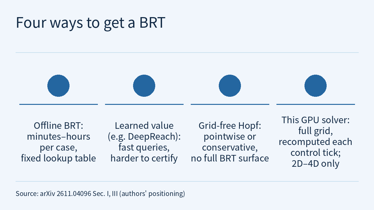
The difficulty is that level-set computation on a grid grows exponentially with state dimension. The usual practice has been to compute the BRT once offline (the paper says prior work typically pays minutes to hours per case) and use it as a fixed lookup in the control loop. The authors’ argument is that when the disturbance model, the obstacles or the dynamics are not known in advance, a stale BRT is a stale safety guarantee.
The related-work section places the solver among other approaches. DeepReach and similar methods fit the value function with a neural network, which is fast to query but harder to certify; grid-free Hopf-type methods evaluate the value pointwise or give conservative approximations, without the full BRT surface. This paper keeps the full grid and makes the whole-surface solve fast. DualGuard MPPI uses a precomputed BRT as a hard constraint for sampling-based MPC; the authors describe their own work as upstream of that, replacing the precompute with an online recompute.
The solver: same scheme, fused CUDA kernels
The scheme is standard: fifth-order WENO5 gradient reconstruction with a six-cell stencil per dimension, a Lax–Friedrichs numerical Hamiltonian (global, local and local–local variants), third-order TVD Runge–Kutta time integration, and a time step that keeps Δt·α_max/Δx ≤ 0.75. After each time step Mitchell’s BRT clamp V ← min(V_new, V_old) keeps V non-increasing under backward integration. The authors attribute the speed-up to structure the discretization itself exposes:
- One fused kernel per RK3 stage. WENO5 reconstruction, the Hamiltonian, the stage combine and, on the last stage, the BRT clamp all run in registers, so the stage right-hand side never goes through global memory; the third stage writes V in place, removing a copy per step.
- One division per WENO5 reconstruction. The weight normalization is rewritten algebraically so that one reconstruction needs 1 division instead of the textbook 13, identical up to round-off. The authors note that consumer GPUs execute FP64 division in software and that
--use_fast_mathdoes not apply to doubles. - The CFL step is computed once on the host. For every Hamiltonian in the paper the wavespeed bound is time-invariant, so no full-grid reduction is needed per stage.
- Stencil values come straight from L2 cache. At control-rate grid sizes the field fits in L2 (101³ FP32 values are about 4 MB against a 40 MB L2). The authors measured a shared-memory-tiled 3D stencil at roughly one third the throughput of direct fetches.
- The 3D solver records a whole step as a CUDA graph and replays it. Precision is a template parameter switching between float and double; the FP32 mode targets embedded deployment.
As a baseline the authors also wrote a PyTorch implementation of the same scheme compiled with torch.compile. Their explanation is that the items above are algebraic identities and dataflow facts about the discretization that a general tensor compiler cannot assume under IEEE semantics. They also state that the torch.compile route is easier to write and modify and brings automatic differentiation.
Matching the reference before talking about speed
The reference implementation is Stanford ASL’s JAX library hj_reachability. Eight cases (2D holonomic, double integrator, three wind-affected drifters, 3D Air3D, two 4D pursuit–evasion cases) are defined in shared JSON specifications, both sides using WENO5, TVD-RK3, CFL 0.75 and FP64. The two clamp operators differ: this solver clamps once per full RK3 step, while hj_reachability clamps the Hamiltonian in each substage; the authors state that the reported agreement was measured with this difference in place.
- Pointwise L∞ difference at the largest matched grid: 0.00217–0.0130 for the 2D cases, 0.0223 for Air3D and 0.347 for 4D pursuit–evasion (V spans about 2.6). The authors attribute the difference mainly to smearing of the non-smooth BRT boundary rather than to truncation error in smooth regions.
- For Air3D (t = 2 s, both vehicles at 5 m/s, maximum turn rate 1 rad/s, 5 m collision cylinder) at N = 51, the two BRT cell counts differ by 4 out of about 11,200, or 0.04%.
- For 4D pursuit–evasion with default settings, this solver’s BRT is 7.1–7.5% smaller than the reference. The authors trace the gap to two scheme choices: a gradient-local Lax–Friedrichs coefficient and linear extrapolation at non-periodic boundaries. With both aligned, the cell counts differ by 0.6%, 0.4% and 0.3% at N = 31, 41 and 51.
- FP64 single solves are 2.0–4.6× faster than JAX and 1.3–1.4× faster than
torch.compileon the six distinct dynamics; at the same L∞ accuracy target they are 3.1–4.9× faster than JAX-GPU.
Read the real-time numbers together with grid and precision
The closed loop uses FP32. The authors report that on the RTX 4000 Ada FP32 is 21–33× faster than their own FP64 path; the FP32 BRT is cell-for-cell identical to FP64 on the 2D and 3D cases and differs by at most 0.1% of cells on the 4D cases. The table below is taken from Table IV of the paper; “rate” is the reciprocal of a single solve time:
| Case | Dim. | N | This solver (ms) | Rate | JAX (ms) | torch.compile (ms) |
|---|---|---|---|---|---|---|
| air3d | 3D | 51 | 8.91 | 112 Hz | 52.3 | 50.0 |
| air3d | 3D | 101 | 102 | 9.8 Hz | 804 | 178 |
| drifter_const | 2D | 200 | 6.82 | 147 Hz | 86.4 | 107 |
| drifter_wg | 2D | 200 | 13.6 | 74 Hz | 159 | 223 |
| pe_4d | 4D | 31 | 16.4 | 61 Hz | 150 | 27.6 |
| pe_4d | 4D | 51 | 222 | 4.5 Hz | 3885 | 573 |
For the same Air3D case, raising N from 51 to 101 drops the rate from 112 Hz to 9.8 Hz; for the same 4D pursuit–evasion case, N = 31 gives 61 Hz and N = 51 only 4.5 Hz. According to the sweep in Fig. 3 of the paper, the FP32 solves that fit a 30 Hz budget are Air3D up to N = 71 (36 Hz), 4D pursuit–evasion up to N = 31 and the 2D drifter up to N = 200; those that fit a 100 Hz budget are Air3D up to N = 51 and the constant-wind drifter up to N = 200. On the same hardware and both in FP32, this solver is 5.9–17.5× faster than hj_reachability (Table IV), 5.7–17× across the whole sweep (Fig. 3), and 1.7–16× faster than torch.compile.
The same source is built for a Jetson AGX Thor developer kit (T5000 module, 2560-core Blackwell GPU, 128 GB LPDDR5X unified memory, 120 W power-mode cap). The authors report single solves 2.7–3.5× slower than on the desktop: Air3D 15.1 ms (66 Hz) at N = 41 and 28.9 ms (35 Hz) at N = 51; the drifter at N = 200 18.6 ms (54 Hz) with constant wind and 37.1 ms (27 Hz) with spatially varying wind; 4D pursuit–evasion 53.9 ms (19 Hz) at N = 31. On the same device it is 3.8–8.9× faster than hj_reachability, but the JAX baseline there uses XLA’s default, untuned fusion configuration, because the autotuner of jaxlib 0.10.0 cannot run on sm_110.
Multi-agent demonstration: one solve for a six-drone partition
The paper uses a simulated demonstration to show what problem an online solve can serve: six identical quadcopters defend a 20 × 20 km region at a cruise speed of 20 m/s under wind that varies in time and space (a 12 m/s background wind that rotates from NE to NW over the 15-minute simulation, plus a cyclonic rotor whose tangential speed reaches 30 m/s during an 80-second gust window around t = 500 s). At every 10 Hz outer-loop tick it recomputes, from each drone’s current position, which drone can reach each cell first, that is, the capture-basin Voronoi tessellation for a 10-minute horizon; cells no drone can reach within the horizon are marked separately. When a fire appears, the label of its cell decides dispatch; if the cell is unreachable, or its owner is busy with another fire, the fire waits.
The method uses the min-preservation property for identical agents: the minimum of the drones’ time-to-reach fields satisfies the same HJ equation, so a single combined solve is enough, with an integer label propagated inside the kernel; each cell the front has just reached inherits the label of its labelled neighbour with the smallest V. The authors report that the labelled combined solve costs about 1.3× a single-agent solve. With K = 6 on a 200 × 200 grid, the combined solve takes 15–17 ms against 69–77 ms for six separate solves (4.6×); labels agree with a per-agent argmin reference on 99.5% of cells, the disagreement being a one-cell stripe along the bisectors. In the closed-loop simulation each tick takes 4.0 ms (mean over 9,000 ticks), and all three fires are suppressed within the simulation. On Thor a tick takes 9.69 ms with clocks pinned at an average system input power of 34.4 W, and 10.35 ms at 31.1 W under default dynamic clocking.
This demonstration uses the first-order mode (RK1 plus upwind), not the high-order WENO5 + TVD-RK3 scheme above; the wind field is treated as known; and what it demonstrates is dispatch, not safety filtering.
How it relates to this site’s course
Physical AI Lab 2.7: Safety Filters uses a control barrier function (CBF): a hand-written h, with the filter as a small quadratic program with a single constraint. HJ reachability takes a different route: the safe set is not written by hand but computed from the dynamics and the disturbance set, at the cost of the grid computation this paper is trying to cut down. In its related work the paper mentions two other ways to plug in a BRT: as the terminal safe set of an MPC predictive safety filter, or as a hard constraint for MPPI. Lesson 2.7 stresses that the guarantee is relative to the model. This site’s reading is that the same holds for a BRT: if f(x, u, d) or the disturbance set in the equation is wrong, the tube is wrong however fast it is computed. The paper envisions recomputing the BRT under the current friction coefficient, contact model and so on, which requires current estimates of those quantities first; the text this site read does not discuss where those estimates come from.
Physical AI Lab 2.6: To the Edge showed that the ceiling on control rate is the reciprocal of the latency of one loop. The 112 Hz in the table is only the reciprocal of one solver call; in a real loop, state estimation, handing the new V to the filter, and actuation add to it. The paper reports single-solve times and the tick time of a simulated closed loop; it gives no end-to-end latency for a safety-filter loop on a real robot.
Limitations
- This is an arXiv preprint and every number is author-reported [R]; this site has not reproduced any of them. The paper describes the solver as a C++/CUDA library with no Python runtime, but the text this site read (the references are cut off at entry 13) gives no code address.
- The paper contains no closed-loop safety-filter experiment. In its future work the authors write that the most direct test of their central claim would be a quantitative closed-loop study of an online-recomputed BRT as a safety filter, compared on the same robot with offline-precomputed and neural-approximator baselines in a task where the disturbance model shifts during the mission. VLA, humanoid and ADAS uses are application ideas listed by the authors, not experimental results.
- The dimensional ceiling is unchanged. The authors state that the exponential growth with state dimension is not changed by this work; only the constants move: in FP32 a 4D solve on 51⁴ ≈ 6.8 × 10⁶ cells takes 0.22 s, nearly 7× the 30 Hz budget, while the 31⁴ grid solves in 16 ms but at coarse spatial resolution. Above 4D, the authors consider state-space decomposition or learned value-function approximations still the appropriate tools.
- FP32 and FP64 differ by up to 0.1% of cells in 4D. The authors recommend treating a thin band along the BRT boundary as a region of uncertain classification rather than a hard boundary. A grid BRT is itself a numerical approximation.
- Desktop numbers come from one RTX 4000 Ada (20 GB, 130 W TDP); Thor numbers are medians of 7 runs with clocks pinned on an idle host; the JAX baseline on Thor is untuned.
- The wildfire demonstration is a simulation in first-order mode with a known wind field. The authors also note that each tick currently re-allocates and re-uploads the static flow field.
- The paper’s acknowledgment states that generative AI (Claude) was used extensively in preparing it, for drafting text and for writing and optimizing the CUDA/C++ solver and the benchmarking and figure code; the authors state that they reviewed all text and code and re-ran every reported measurement.
- None of these results is a hardware safety validation.
Links
- Online Hamilton–Jacobi Reachability Onboard the Robot Control Loop: A Real-Time GPU Solver for Safety-Critical Autonomy (arXiv 2611.04096)
- Full paper in HTML
- Physical AI Lab 2.7: Safety Filters — Working Out One Control-Barrier-Function Correction by Hand, Then Choosing Its Loop and Its Safety Margin
- Physical AI Lab 2.6: To the Edge — Working Out the Control-Rate Ceiling from a Latency Log, Telling Whether Quantization Saves Size or Time, Then Sizing an Action Chunk
- Physical AI Lab: a physical AI course where every number can be checked (course outline)