Lesson video
Narration is AI-generated. Video chapters, transcript and sources
Transcript
Transcript
UNIT-01 asks
The same model flies on a computer. So why, once it's on a robot, does it fall behind its own hands and feet? Last time, we tuned our policy in simulation. This time, we move it onto a real robot. There's no way around three words: quantization, latency, and control rate.
Latency and control rate
First, one iron rule. In every control cycle, the robot first gets its current observation. Then it computes the next action, and sends it to the motors. How long does one computation take? That decides how many times per second it can run, at most. Latency and rate are two sides of one coin. How fast is low-level control? One paper says the control loop must run a thousand times a second. It treats that as the floor for real-time control. Latency is made of several pieces. Reading the image, preprocessing, model inference. And finally, sending the action out. Then there's communication. Sensor to computer, computer to motor, it all travels down wires. Added up, those pieces can't be ignored either. Behind this is a hard real-time requirement. Every single step must be delivered on time. Miss by a hair, and it can all be for nothing. Why does it have to be so fast? One beat late, and the contact force overshoots. Either things slip, or they get broken. Put another way. In the time it takes you to blink, it has quietly corrected itself many times over. Too fast for you to ever see. And large models? A vision-language-action model thinks far more slowly. In a measurement by Amazon, one such model can re-plan about five times a second. Put the two side by side, and the rates differ by more than two orders of magnitude. That's not a figure of speech. It's a real gap. So that's what "the brain thinks slowly, the cerebellum moves fast" means! The difference is the rate. Here's another trap. Real systems don't care about average latency. They care about the worst moment, the tail latency. An occasional hiccup barely shows in the average. But that one moment might be when the robot falls. So keep your eyes on the worst case. To speed things up, first find the slowest piece. Very often, it's model inference. So that's where we start.
Quantization: shrink the model
How do we get a model running on a small device? Trick one, quantization. Use fewer bits to store and compute. What does that mean? Map a wide range of continuous values onto a few integer levels. And remember one scale factor to restore them anytime. We use dynamic quantization. The weights are compressed to eight-bit integers first. The activations are quantized on the fly, during inference. First, size. PyTorch says that switching to eight-bit integers makes a model four times smaller. That's the most reliable gain. Next, speed. The same official blog says inference gets two to three times faster. But it depends on the hardware and the model. Let's be precise, not hype it. In this episode's notebook, the model really is four times smaller. But on this CPU, it actually got slower. Why? This network is tiny, and it runs on a CPU. The extra overhead of quantization outweighs the computation it saves. So when does it speed things up? When the model is big enough, and stuck on memory bandwidth. Integers move fast, and compute fast. There's another reality. Memory on edge devices is often painfully small. It has to fit before it can run. How much accuracy loss you can live with depends on the task. Grabbing a cup? Maybe it doesn't matter. Surgery? Not the slightest slip. Quantization isn't the only trick. There's also pruning, distillation, and a smaller backbone. They're often used together. But quantization is the easiest. One line of code swaps the linear layers for integer versions. That's why we cover it first. Quantization has a cost too. It's an approximation at heart, so accuracy drops a little. Luckily, usually only a tiny bit. So quantization isn't magic. Saving space is the sure thing; speed-ups depend!
To the edge, and running for real
With the size down, it still needs somewhere to compute. NVIDIA describes a robot computing module that can run the latest models within one hundred thirty watts. Why compute on the robot itself? The cloud means a round trip, high latency, and the risk of losing the network. And you may not want camera data leaving the robot. But no chip is fast enough to run a large model at every single step. There's no getting past the latency barrier. The engineering fix is to separate the slow from the fast. Let the large model think at a low rate. Each time, it plans a whole stretch of motion. Then hand it to a very fast controller, which carries it out step by step. This is called action chunking. Action chunking takes care too. Chunks too long, and it can't react to anything new. Chunks too short, and you're back to the old problem. So you have to strike a balance. Think far enough ahead, without losing your reflexes. That's the craft of edge deployment. Splitting slow from fast brings a bonus, too. Jobs like safety checks can live inside that fast loop. Step by step, catching every action. So the key isn't making the model faster. It's keeping it out of the fast loop! This way, the slow planner thinks at its own pace. The fast controller moves at its own pace. Two rates, each in its own lane. What's still unsolved? Latency has only shrunk, not vanished. When the network jitters, one chunk may not connect to the next. That's when something has to catch it. Open this episode's notebook and follow along. Measure the latency once before quantization and once after. Then turn it into how many hertz it can run at. You'll see that iron rule with your own eyes. One over the latency is the ceiling on the control rate. Numbers don't lie. Let's recap, three points. One, latency sets the upper limit on rate; they're reciprocals. Two, quantization's most reliable gain is size; speed-ups must be measured. Three, pair slow planning with fast control, decoupled by chunking. Bringing a large model down from the cloud and onto a robot doesn't take a faster chip. It takes a smarter division of labour! But what if the model computes a dangerous action? Who stops it? See you next time!
Evidence and sources
Practice and self-check
- Interactive quiz5 questions, explained as you answer
- One-page summaryprintable; opens in a new tab
- Download the notebookszip in Chinese, English and Japanese; run in Jupyter or upload to Colab
The quiz is public and explains each answer as you go; answers to the guide's exercises are for signed-in members.
The episode 2.6 video takes the policy tuned in simulation in the previous episode onto a robot and makes three points: the ceiling on control rate is the reciprocal of the latency of one cycle, and a real system has to watch tail latency, not the average; quantization’s surest gain is size (int8 shrinks a model to about a quarter), while any speed-up depends on the hardware and has to be measured; a large model thinks slowly while low-level control must be fast, so engineers separate the two with action chunking, and latency is managed rather than eliminated. The video’s four number cards come from four public sources. The multipanda_ros2 paper (arXiv 2602.02269) says sustaining a 1 kHz control frequency is a necessity for its real-time control and a minimum frequency required by safety standards. An AWS blog reports that π0, at 1 ODE step on an H100, produces a 50-step action chunk in under 200 ms and can re-plan at about 5 Hz. A PyTorch blog says quantization gives a 4x reduction in model size and a 2x to 3x speedup, depending on hardware and model. An NVIDIA blog says Jetson Thor delivers up to 2070 FP4 TFLOPS of AI compute within a 130 W power envelope. This page is the episode’s reading and exercises. It does not repeat the transcript; it does three things the video only touches on. It puts the four numbers back in their own systems, separating the one about a control loop, the one about a planner, the one about model size and the one about power. It works through stage latencies, rate ceiling and overruns with a set of hypothetical numbers. And it splits “what quantization saves” into three accounts, weight size, runtime memory and latency, before choosing a re-planning period and chunk length for a slow planner. The rule throughout: a rate, latency or multiple belongs only to the system, hardware and set-up that measured or specified it; numbers from different systems cannot be multiplied or divided together, or assembled into one robot’s specification.
The video, transcript and sources for this lesson are at the top of this page; the season plan is in the course outline. The previous lesson, Physical AI Lab 2.5: Sim2real with Domain Randomization and System Identification — Putting Two Papers’ Numbers Back in Their Setups, Then Working Out Friction by Hand from One Push of a Cup, ended by asking: with the parameters matched, what do latency and compute hold back once the model is on the robot? This lesson takes up that question. Which system each of three rates belongs to was practised in Physical AI Lab 0.3: See, Think, Act — Putting Each Rate Back in Its Own System; turning rates into periods was worked out in Physical AI Lab 1.2: PID and Control Rate — Computing the Three Terms by Hand, Then Turning Rates into Periods; Jetson Thor’s compute multiple over the previous generation was covered in Physical AI Lab 0.2: Why Now? The Three Curves of Data, Models, and Compute; the timing margin of an action queue under asynchronous inference was worked out in Physical AI Lab 2.3: Fine-Tuning SmolVLA — Planning Demonstrations for an Instruction, Checking What Each Number Measures, Then Timing the Asynchronous Action Queue; and pairing success rates and classifying failures were practised in Physical AI Lab 1.8: Evaluation — Splitting a “Net Gain of 2” into a Paired Table, Then Checking the Failure Labels and Random Seeds. This lesson does not repeat those. It covers only the four sources new to this episode and the accounts that latency, quantization and action chunks require. How safety checks hook into the fast loop is the subject of the next episode, 2.7 (control barrier functions).
The public quiz’s 5 questions come with full explanations. Signed-in readers can work three exercises: from a fictional 20-cycle latency log, work out the rate ceilings implied by the median, the mean and the worst case, and count overruns at three target rates; read a fictional quantization benchmark, keeping weight size, runtime memory and latency in separate accounts, and judge four claims; review a fictional edge deployment plan, choose a re-planning period and chunk length for a slow planner, and rewrite the sentences that cite three sources. Each comes with a step-by-step worked solution, common mistakes and a 20-point rubric.
1. Four numbers, four systems
The video’s four number cards correspond to four sentences in the originals, quoted separately below. In this course’s grading the paper is level R and the three vendor or official blogs are level O; all the numbers are reported by the authors or vendors, and this site has reproduced none of them.
The multipanda_ros2 paper (Škerlj et al., arXiv 2602.02269; the page notes a published version at ICRA 2026), abstract:
A central focus of this work is sustaining a 1kHz control frequency, a necessity for real-time control and a minimum frequency required by safety standards.
The AWS blog Fine-Tuning π0 (Pi-Zero) for robotic manipulation on Amazon SageMaker HyperPod EKS:
At 1 ODE step on H100, a full 50-timestep chunk takes under 200 ms, so the policy can re-plan at about 5 Hz while each chunk covers roughly one second of robot motion.
The PyTorch blog Introduction to Quantization on PyTorch:
Quantization provides a 4x reduction in the model size and a speedup of 2x to 3x compared to floating point implementations depending on the hardware platform and the model being benchmarked.
The NVIDIA technical blog Introducing NVIDIA Jetson Thor, the Ultimate Platform for Physical AI (2025-08-25):
Jetson Thor delivers up to 2070 FP4 teraflops of AI compute within a 130 W power envelope.
| What the video says | Whose number it is | Conditions in the original | What the original does not say | Level |
|---|---|---|---|---|
| A thousand times a second, the floor for real-time control | multipanda_ros2: an open-source ROS 2 framework built on ros2_control that controls several Franka Robotics robots from a single process | Its real-time torque control loop; section II says a 1 kHz low-level torque command loop lets higher-level controllers treat the joints as ideal torque sources, and says safety standards such as ISO 10218 specify 1 kHz measurement frequencies for collision detection | It does not say a planner or VLA must run at 1 kHz; this lesson did not consult the text of ISO 10218 | R (author-reported) |
| Re-plans about five times a second | π0: Physical Intelligence’s 3-billion-parameter VLA; the blog uses the LeRobot port lerobot/pi0_base | One H100, 1 ODE integration step, under 200 ms per 50-step action chunk, each chunk covering about one second of robot motion | Not a measurement on an edge device; the blog’s accuracy evaluation averages only the first 5 held-out episodes | O (vendor’s own measurement) |
| Four times smaller, two to three times faster | PyTorch int8 quantization; the blog dates from when PyTorch 1.3 introduced quantization and 1.4 published quantized models | Compared with floating-point implementations; the speed-up depends on the hardware platform and the model benchmarked | No speed-up is guaranteed for any given model; the 4x is size, not speed | O (official blog) |
| Runs the latest models within a hundred and thirty watts | Jetson Thor; in the spec table, the Jetson T5000 module | Up to 2070 FP4 TFLOPS (the spec table says Sparse FP4); power range 40–130 W | Not the latency of any model on a robot; 2070 is a peak compute figure | O (vendor’s description) |
Four things to note when reading this table:
- About 5 Hz is itself a reciprocal. The blog derives “about 5 Hz” from “a chunk takes under 200 ms”: 1 ÷ 0.2 s = 5 per second. It is the ceiling on how often this planner can re-plan on this hardware, not the rate of the robot’s low-level loop. The same blog also reports that on LIBERO, going from 10 ODE steps to 1 cuts latency from 379 ms to 197 ms with no accuracy cost. Quantization is not the only way to save time.
- “More than two orders of magnitude” sets two systems side by side. The video places about 5 Hz next to 1 kHz to show how far apart a large-model planner and a low-level torque loop are in rate; the 5 Hz comes from π0 on an H100 and the 1 kHz from a Franka multi-arm framework, so the gap is not a ratio measured on one robot. The π0 paper figure used in 0.3 (on a robot running at 50 Hz, re-running inference after every 25 actions, about every 0.5 s) is yet another set of conditions and cannot be merged with AWS’s figure.
- 1 kHz is not a parameter every robot shares. In the paper’s Table I of torque-controlled robots, most command rates are 1 kHz, but Boston Dynamics Atlas 1 (2013) is listed at 333 Hz and Berkeley Blue (2019) at 170 Hz; the authors describe the list as non-exhaustive.
- The 130 W sentence comes from the summary at the top of the page that is labelled as AI-generated. The corresponding sentence in the body says the developer kit, powered by a Blackwell GPU and 128 GB of memory, delivers up to 2070 FP4 TFLOPS to run the latest generative AI models, all within a 130 W power envelope; the spec table lists the T5000 module’s power as 40–130 W. These are the vendor’s descriptions of hardware capability and say nothing about the latency of any model running on it.
Sign in to keep reading: the rest of this lesson, its self-check questions and the answers.
Limitations
- multipanda_ros2 (arXiv 2602.02269) is level R, and its page notes a published version at ICRA 2026; the 1 kHz, the rates in Table I and the statement about ISO 10218 are the authors’ statements. This lesson read the abstract up to the start of the methods section; it did not consult the text of ISO 10218 or read the paper’s experimental results.
- The AWS blog is level O, a vendor measurement under its own set-up: the LeRobot port of π0, one H100, 1 ODE step; the accuracy evaluation covers only the first 5 held-out episodes. This site has not reproduced it.
- The PyTorch blog is level O and dates from the PyTorch 1.3 and 1.4 period; its API names, backend support and sample numbers apply to that release, and this lesson did not check later versions.
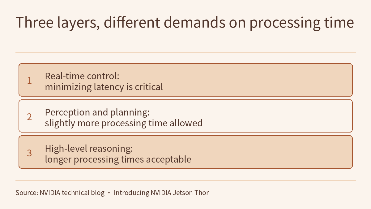
- The NVIDIA blog is level O. The 130 W sentence used in the video comes from the summary on the page labelled as AI-generated; the body and the spec table say the same. 2070 FP4 TFLOPS is a peak compute figure, and the spec table marks the T4000 figures as preliminary. The four layers are the vendor’s description of a typical humanoid robot, not a standard, and come with no milliseconds; the diagram omits the hardware abstraction layer, for which the original gives no time requirement.
- The Notebook result in the video (“four times smaller, but slower on a CPU”) is reported only as the video states it; this lesson did not run the Notebook or read its saved latencies.
- The following are this lesson’s notes, modelling choices or inferences, not statements in the originals: the assumption that a cycle runs in series, and the note about pipelining; the model in which the worst-case reaction time is about P + L (plus the round trip) and the conservative rule that a chunk must cover at least P + worst L; the suggested measurement and evaluation practices; the arithmetic with 1 MB = 10⁶ bytes and scale factors ignored; and reading AWS’s “not memory-bound” as referring to VRAM capacity, based on the sentence that follows it.
- Robots R and R6, policy networks S, Q and T, devices A and E, planner V, team W, and all latencies, parameter counts, memory sizes, errors, round-trip times and task requirements in sections 2 to 5 are fictional; 20.8 Hz, 25 Hz, 1.83 times, 0.72 s and the like hold only under these assumptions.
- Calculations on paper and simulation results are not hardware safety validation; fallback behaviour on overruns and gaps needs its own safety analysis, and trials on a real robot need their own safety preparation.
Links
- Physical AI Lab: a physical AI course where every number can be checked (course outline)
- Physical AI Lab 2.5: Sim2real with Domain Randomization and System Identification — Putting Two Papers’ Numbers Back in Their Setups, Then Working Out Friction by Hand from One Push of a Cup
- Physical AI Lab 2.3: Fine-Tuning SmolVLA — Planning Demonstrations for an Instruction, Checking What Each Number Measures, Then Timing the Asynchronous Action Queue
- Physical AI Lab 1.8: Evaluation — Splitting a “Net Gain of 2” into a Paired Table, Then Checking the Failure Labels and Random Seeds
- Physical AI Lab 1.2: PID and Control Rate — Computing the Three Terms by Hand, Then Turning Rates into Periods
- Physical AI Lab 0.3: See, Think, Act — Putting Each Rate Back in Its Own System
- Physical AI Lab 0.2: Why Now? The Three Curves of Data, Models, and Compute
- Frontier Radar deep dive | Edge and real-time: where the latency budget of VLAs and world action models goes (millisecond figures from another 9 sources in the radar’s September archive)
- Bridging the Sim-to-Real Gap with multipanda_ros2: A Real-Time ROS 2 Framework for Multimanual Systems (arXiv 2602.02269)
- AWS: Fine-Tuning π0 (Pi-Zero) for robotic manipulation on Amazon SageMaker HyperPod EKS
- NVIDIA technical blog: Introducing NVIDIA Jetson Thor, the Ultimate Platform for Physical AI (2025-08-25)
- PyTorch blog: Introduction to Quantization on PyTorch