The preprint ODE Policy (arXiv 2611.01729, 2026-11-01, MARS Lab, Nanyang Technological University) changes what a robot policy outputs. Instead of producing the action value at each control step, the network learns how fast the action changes, that is, the action’s vector field, and integrates each action from the previous one. The executed action trajectory is therefore continuous by construction, and consecutive action chunks do not jump at their boundaries. The authors use the same formulation as a visuomotor policy, as the action head of π0.5 and ImageWAM, as the action head of GR00T N1.7 on a humanoid, and as the RL actor of SuperMimic. When reading the results, note that the largest advantage appears early in training; in several settings the baselines later caught up. All numbers below are author-reported [R]; this site has not reproduced them.
What direct-action policies leave out
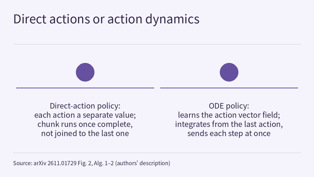
The paper calls existing policies “direct-action policies”: they encode the observations and the proprioceptive state and output the values of future actions directly. Whether the head is a regressor, a diffusion or flow matching generator, or an RL actor, each action is a separate value, the model itself imposes no relation between consecutive actions, and the continuity of motion must be learned implicitly from data. The authors point to three consequences:
- Independently predicted chunks can be inconsistent at their boundaries, so the commands jump.
- Diffusion and flow matching do solve a differential equation at inference, but the integration variable is a “generation time” with no physical meaning; intermediate samples are not states the robot can occupy, and each chunk is generated anew, regardless of where the previous one ended. Generative policies also need several network evaluations per chunk, and the first action can run only after the whole chunk is generated.
- In RL, without explicit regularization, the actor’s actions often oscillate at high frequency between control steps.
The starting point is that a robot is a macroscopic system that moves continuously in time, and a teleoperated demonstration is largely a sampling of a continuous action trajectory at the control frequency. The paper also notes that methods describing robot motion with ODEs, such as dynamical movement primitives, have a long history, but they fix the form of the vector field or force it to converge to an attractor, so each model covers only a few motions; ODE Policy places no structural constraint on the vector field and learns one field for large-scale tasks.
How it is trained and run
Vector field. The image history and the instruction are encoded into z_t, and a network f_θ(a(t), s_t, z_t) outputs the velocity of the action. Time t is counted in control steps and is the robot’s physical time; the proprioceptive state s_t enters the vector field directly rather than being encoded together with the observation. What gets integrated is the target action sent to the low-level controller, not the measured robot state.
Chunked integration and path loss. z_t is computed once per decision step and held fixed over the chunk, and the chunk is obtained by integrating H steps from the previous action â_{t−1}. In training, the policy integrates H steps from the demonstrated action and uses the squared error between the integrated path and the demonstration as the loss. Because the chunk is short, the gradient is back-propagated directly through the solver steps without the adjoint method; the vector field is also never regressed against velocity labels derived from the demonstrations, which the authors say may amplify the jitter in demonstrations.
Contractive perturbation. At execution, the policy integrates from its own previous output, so errors carry into the next step and the next chunk and the state gradually leaves the demonstrations. In training, with probability p, the start point is shifted by a Gaussian perturbation δ and the integrated path must return to a_{t+k} + ρ^{k+1}δ at step k (0 < ρ < 1). The deviation shrinks geometrically, so the vector field learns to pull nearby states back to the demonstration. This relies on the vector field taking the current action as input, and the authors note that direct-action policies have no counterpart. It needs no additional data and no additional computation at inference.
Inference. Each action is obtained from the previous one by one integration step, and the next chunk continues from the last action of the previous chunk rather than restarting from the measured state; the paper calls this seamless chunking. The authors list three benefits: chunks join without jumps; each action can be sent to the controller as soon as it is integrated, without waiting for the whole chunk; and the integration step can be chosen at deployment, for example to match a higher control rate.
Diversity head. A deterministic vector field fits the mean velocity of the demonstrations, so demonstrations that pass an obstacle on the left and on the right get averaged into heading straight into it. The authors add a lightweight head: at the start of each chunk it samples a direction ε from a K-component Gaussian mixture and a non-negative rate λ_k for each step, and adds λ_k ⊙ ε to the velocity. It reads the vector field’s hidden features with the gradient stopped and leaves the vector field’s gradient unchanged. The authors also note that strong multi-modality occurs in only a small part of tasks: on LIBERO, actions for the same observation differ only slightly, and although all IL experiments include the head, on LIBERO it uses the component mean rather than sampling.
RL. The actor produces one action per control step (H = 1) by taking one Euler step from the previous action: â_t = â_{t−1} + f_θ(…). The critic and the algorithm are unchanged. SuperMimic backpropagates the return through 32 imagined steps, and this step makes ∂â_t/∂â_{t−1} contain the identity, so the gradient can reach early actions along the chain of actions.
Results: read them by training epoch
The abstract summarizes that in imitation learning, against flow matching, the method reaches 5.9 times the success, 5.4 times the generalization and 3.9 times the mode balance after one epoch, and generates actions 10.8 times faster. The details in the body show that the first three ratios are concentrated early in training (10.8 times is inference speed and does not depend on the training epoch):
| Setting | After 1 epoch | Later |
|---|---|---|
| Visuomotor policy, four LIBERO suites (3 seeds) | 79.2%; best of 6 baselines 43.2% | Passes 85% at epoch 2, still leads at epoch 100 |
| π0.5 action head (1 seed) | 96.0%; randomly initialized FM expert 75.5% | The FM expert initialized from π0.5’s pretrained weights catches up from epoch 2 |
| ImageWAM action head (1 seed) | 82.6%; original head 24.6% | All three heads converge from epoch 6 |
| LIBERO-plus zero-shot perturbations (visuomotor) | 30.1%; ACT 22.6% | Later on par with the strongest baselines |
| 2D navigation with four routes, mode balance γ | 3.9 times FM-DiT | FM-DiT more balanced at epoch 10; similar at epoch 20 |
The abstract and introduction say “96.0% against 75.5% for its flow matching expert”; Section 6.1.2 makes clear that 75.5% is the randomly initialized FM expert. The ODE head has about 13.7M parameters and replaces the original 430M action expert (about 3%, according to the paper), and it is also randomly initialized.
The data and parameter results also come from LIBERO: with 20 demonstrations per task, the method reaches 87.7% at epoch 100, above FM-DiT trained on all 50 (85.4%); with only 1.5M parameters outside the encoder, it reaches 92.5% at epoch 10, above the 48M FM-DiT at any epoch (at most 87.5%). The authors conclude that the advantage comes from the ODE formulation, not from model capacity.
On speed, with Euler a chunk of 8 actions takes 5.7 ms, as fast as A2A-DiT, 10.8 times faster than FM-DiT and about 100 times faster than DDPM; ACT is slightly faster but at a much lower success rate. In π0.5, the ODE head runs about 14 times faster than the FM expert with 10 denoising steps and saves about a third of the full model’s time; at chunk boundaries, the commands change about half as much. In ImageWAM, the time per chunk falls to about a quarter.
Fourteen real-robot tasks and RL
The real-robot part uses four robots: a single-arm Franka Research 3, a dual-arm Galaxea R1 Lite, a Sharpa North with a Sharpa dexterous hand, and a Unitree G1 humanoid with Inspire DFX dexterous hands. Each task is evaluated with 20 trials; training runs for 300 epochs by default, only 50 on the single arm (deliberately, to test early performance) and 90 on the humanoid. The baselines differ from robot to robot. The authors report that ODE Policy has the highest success rate on all 14 tasks; some of the results:
- Single arm (40 demonstrations per task): folding a sock 15/20 and inserting a block 14/20, against 8/20 and 4/20 for the best baseline.
- Dual arm: on the microwave task, learned from only 34 demonstrations, 75% against 20% for FM-DiT; on the multi-modal drawer task, where either arm may place the apple, the left arm went for it in 8 trials and the right in 12, with 60% success overall, while FM-DiT went for the apple with both arms but never placed it.
- Dexterous hand: trained only on public SharpaDex data from another lab (50 demonstrations per task) and deployed in the authors’ lab, reorienting a fallen cup 17/20 (FM-DiT never grasped the cup), pouring pills with two hands 17/20 (FM-DiT 10/20), and stacking cubes 13/20 (both baselines always failed).
- Humanoid: as the action head of GR00T N1.7 (a vector field of about 5M parameters, H = 16, Euler), with 90 demonstrations per task, 60% and 70% on two long-horizon tasks that combine walking and grasping, against 35% and 30% for GR00T’s original head.
With 20 trials per task, one trial equals 5 percentage points (this site’s arithmetic); the text read gives no confidence intervals for the real-robot results. On one task on each of three robots, a chunk is generated 3.5–27 times faster than with the diffusion and flow matching baselines; command acceleration at chunk boundaries stays at or below that of the demonstrations (close to it on the single arm), while the baselines reach several times that of the demonstrations.
In the RL part, the ODE actor replaces SuperMimic’s actor while the world model, critic, rewards and hyperparameters stay the same; a simulated Unitree G1 tracks 40 LAFAN1 motion clips, with 3 seeds per method and 3 hours of training on one GPU. At 0.75 hours, the training return is 37% higher (0.630 ± 0.007 against 0.460 ± 0.008); the evaluation return on all 40 clips is 30% higher at 0.4 hours and ends at 0.885 ± 0.007 against 0.845 ± 0.009; PPO reaches 0.452 ± 0.021 after 3 hours. The gradient norm with respect to the first imagined action, relative to the last, is about 0.57 for the direct-action actor and 1.0–1.1 for the ODE actor; the authors say the speed-up “likely” stems from this gradient path. After 3 hours, the ODE actor’s actions accelerate 21% less than those of the original actor.
Which design choices matter: ablations
- Chunk length. With H = 1 in training and execution, the policy reaches only 76.4% at epoch 100 and is the slowest per action (the encoder runs at every step); from H = 4 on, success stays above 91%, best at the default H = 8; for H ≥ 12, training shows occasional loss spikes.
- Solver. Replacing RK4 with RK2 or Euler changes success at epoch 100 by less than one percentage point, within the variation across seeds. The authors conclude that the performance comes from the ODE formulation, not from an accurate solver; with Euler, training takes about as long as FM-DiT.
- Contractive perturbation. Without it, success after one epoch drops from 79.8% to 58.4% (this ablation uses 10 episodes per task, hence 79.8% rather than 79.2% for the default), and the gap closes by epoch 20; twice the default magnitude stays slightly lower later on.
- Seamless chunking. Restarting each chunk from the measured state instead lowers success after one epoch from 79.8% to 47.8%. The paper’s explanation is that this discards the lead of the target action over the measured state.
This site’s reading is that these two ablations indicate that a substantial part of the large early lead comes from teaching the vector field to return to the demonstrations during training and from continuing integration from the last command during execution. The paper does not state this attribution; in Section 8 it also notes that even without the perturbation, ODE policy is still well ahead of FM-DiT and A2A-DiT after one epoch. The text read gives the early numbers; the full curves for later epochs are in Fig. 17, whose values this site did not read.
How this relates to this site’s course and Frontier Radar
Physical AI Lab 1.6: Imitation Learning covered two points: behaviour cloning errors carry the robot out of the demonstrations’ coverage, and two correct ways around an obstacle can be averaged into a collision. ODE Policy answers each with a structural change: contractive perturbation teaches the vector field during training to pull drifting states back to the demonstrations, and the diversity head picks a direction at the start of each chunk. It also keeps the action chunking of ACT from 1.6, but uses the chunk as the unit of integration.
In Physical AI Lab 2.3: Fine-Tuning SmolVLA, the action expert uses flow matching to refine noise into a chunk step by step, and asynchronous inference computes the next chunk while the current one runs. ODE Policy’s “streaming execution” is a different thing: within a chunk, each action is sent as soon as it is integrated, and the next chunk continues from where the previous one ended. Physical AI Lab 2.6: To the Edge discussed the trade-off in chunk length; this paper’s H ablation gives numbers for the same trade-off for one specific method, measured only on LIBERO. The actor and return in the RL section can be read alongside Physical AI Lab 1.7: Reinforcement Learning.
Frontier Radar | ActionUNet also targets smooth VLA actions, by adding a temporal U-Net and a continuous decoder on the action features of a frozen backbone; ODE Policy instead replaces the whole action head. Their benchmarks and baselines differ, so the numbers cannot be compared. When reading this paper’s tables, the method from Physical AI Lab 1.8: Evaluation suggests questions to ask: π0.5 and ImageWAM have only one seed, each real-robot task has 20 trials, and how far the early lead carries to the end of training.
Limitations
- This is an arXiv preprint; all numbers are author-reported [R], and this site has not reproduced them. The paper’s front page lists a project page and code, which this site did not open or check.
- The text this site read ends partway through the Section 8 ablations. Section 9 (including how the gap between the target action and the measured state is handled when only measured states are available, and the ablation that integrates the gripper with the vector field) and all appendices and supplementary tables were not read.
- “5.9 times, 5.4 times, 3.9 times” are ratios after one epoch of training. In π0.5, the pretrained FM expert catches up from epoch 2; in ImageWAM, all three heads converge from epoch 6; on LIBERO-plus, the method is later on par with the strongest baselines; on the navigation task, FM-DiT is more balanced at epoch 10.
- The visuomotor experiments use 3 seeds; the π0.5 and ImageWAM results use 1 seed. Each real-robot task has 20 trials, the baselines differ from robot to robot, and on the humanoid the only comparison is GR00T’s original action head; the text read gives no confidence intervals for the real-robot results.
- On LIBERO, the binary gripper command is predicted by a separate classification head (0.27M parameters) and is not integrated by the vector field; on LIBERO the diversity head uses the component mean and does not sample.
- What is integrated is the target action sent to the low-level controller. For data with only measured states (for example, UMI-collected data or human videos), the authors discuss the case in Section 9, which this site did not read.
- On LIBERO-plus, a changed camera defeats all methods; the RL results track motions in simulation only, with no real-robot RL. None of these results is a hardware safety validation.
Links
- ODE Policy: Robot Learning via Action Dynamics, Not Actions (arXiv 2611.01729)
- Full paper in HTML
- Physical AI Lab 1.6: Imitation Learning — Working Out How an Error Rolls Out of the Demonstrations’ Coverage, Then Putting the ACT, Diffusion Policy and Data Scaling Numbers Back in Their Own Conditions
- Physical AI Lab 1.7: Reinforcement Learning — Working Out One Episode’s Return to See How a Reward Gets Gamed, Then Reading the Paper’s Terrain Curriculum and Time-out Resets
- Physical AI Lab 1.8: Evaluation — Splitting a “Net Gain of 2” into a Paired Table, Then Checking the Failure Labels and Random Seeds
- Physical AI Lab 2.3: Fine-Tuning SmolVLA — Planning Demonstrations for an Instruction, Checking What Each Number Measures, Then Timing the Asynchronous Action Queue
- Physical AI Lab 2.6: To the Edge — Working Out the Control-Rate Ceiling from a Latency Log, Telling Whether Quantization Saves Size or Time, Then Sizing an Action Chunk
- Frontier Radar | ActionUNet: a temporal U-Net and a continuous decoder on VLA action features, for multi-scale yet smooth actions
- Physical AI Lab: a physical AI course where every number can be checked (course outline)