The preprint Failure Prediction and Classification in Vision-Language-Action Models via Calibrated Latent Probing (arXiv 2611.08425, 2026-11-05, authors from the University of Texas at Austin, Tufts University and the University of Texas at Dallas) presents VLA-Tug: a small 6.6M-parameter probe on the latent-layer embeddings of a VLA backbone. It aims to raise an alarm before a failure happens, name the likely failure type, and calibrate its threshold so that the false-positive rate and the “early detection rate” are bounded together. The part worth reading closely is how it is evaluated: an alarm counts as timely only against an annotated failure time, and calibration may abstain when a target cannot be met. Read the abstract’s percentages with care: 30% and 44% are relative gains, and the denominator of 86% contains only runs where calibration did not abstain. All numbers below are reported by the authors [R]; this site has not reproduced them.
Three questions a runtime monitor has to answer
The paper breaks a failure detector into a few general concepts. At each control step t there is a failure score s_t (not necessarily a probability in the strict sense) and a threshold h⋆. The detection time t_det is the first time the score crosses the threshold. The failure time t_fail (the authors also call it the failure onset) is when the policy makes an obvious mistake or its progress stalls to the point where a human or another mechanism has to take over; this definition follows SAFE (Gu et al., 2025). A failure mode is a high-level semantic category such as grasping failure, placement failure or no progress. The authors want t_det ≤ t_fail: an alarm before the failure.
The authors see three gaps in existing methods. First, AUROC or balanced accuracy is commonly evaluated at fixed time points, without checking whether the alarm precedes the actual failure time. Second, most detectors output only a scalar risk score without saying which kind of failure it is, so a correction cannot target the cause. Third, calibration usually controls one criterion: it guarantees the false-positive rate (FPR, the share of successful rollouts flagged as failures) but not the true-positive rate (TPR, the share of failures detected). The authors argue that the latter matters at least as much where a single failure could hurt a person or damage equipment. Table 1 of the paper compares SAFE, ActProbe, STAC, FailureSpot and seven VLA steering methods item by item; by the authors’ account, only VLA-Tug combines formal FPR and TPR guarantees, evaluation against failure time and failure-mode prediction.
The probe: which layer it reads, and how failed rollouts are labelled
The input is the latent embedding of the VLA backbone: layer 18 (after normalization) in π0.5 and layer 16 in GR00T-N1.7, the latter being the focus of the analysis. At every policy step, the tokens of each of three modalities (agent camera, wrist camera, instruction) are averaged, and the three 2048-dimensional vectors are concatenated into one 6144-dimensional embedding. A single-layer LSTM with 256 hidden units reads these embeddings in sequence, and three MLP heads, each with one hidden layer of 64 ReLU units, read the same hidden state: a failure score head, a head giving a distribution over 10 failure modes, and an auxiliary head that aligns the hidden state with the CLIP text embedding of the current action’s description. The authors state that at inference this auxiliary head is just a 64-dimensional output and no CLIP encoder runs.
The central hypothesis is that training on post-failure embeddings teaches the probe what already failed trajectories look like, not what trajectories about to fail look like. The authors compare four ways of labelling a failed rollout (every step of a successful rollout is labelled 0):
- pre-onset: every step before t_fail is labelled 1, and steps after it are excluded from the loss. This is what VLA-Tug uses.
- onset: only a window of width w before t_fail is labelled 1, earlier steps are labelled 0, and later steps are excluded.
- post-onset: every step from t_fail − w onward is labelled 1 and earlier steps 0; post-failure steps are kept.
- trajectory: every step of a failed rollout is labelled 1; this is SAFE’s labelling.
The first two truncate at the failure time instead of labelling post-failure steps 0, because those embeddings already belong to a failed rollout, and labelling them as successes would give contradictory training signals. The window w is 2.4 s (6 policy steps for GR00T on LIBERO and 20 on the real robot; 10 steps, or 2.5 s, for π0.5). The authors ablate the labelling in an appendix and report that the other three variants lower early detection on LIBERO-X.
The data are rollouts of two policies, π0.5 and GR00T-N1.7, on three simulation benchmarks (LIBERO, LIBERO-Occ and LIBERO-X) plus real-robot tasks; the paper counts 228 distinct simulated tasks (in two simulation environments) and 8 real-world tasks. Labels are generated from rollout videos by Gemini (gemini-3.5-flash): every rollout gets a keyword timeline in 3-second windows, and failed rollouts also get a failure mode (one of 10) and a failure time. The authors put the labelling cost at about one cent per failed episode, under $50 for all annotations (a total that also includes queries not used in this paper), and release a dataset of 3,180 episodes with over 288,000 backbone embeddings. The main text does not report how well these automatic labels agree with human annotation (at least not in the part this site read).
Early detection: the “30%” is a relative gain
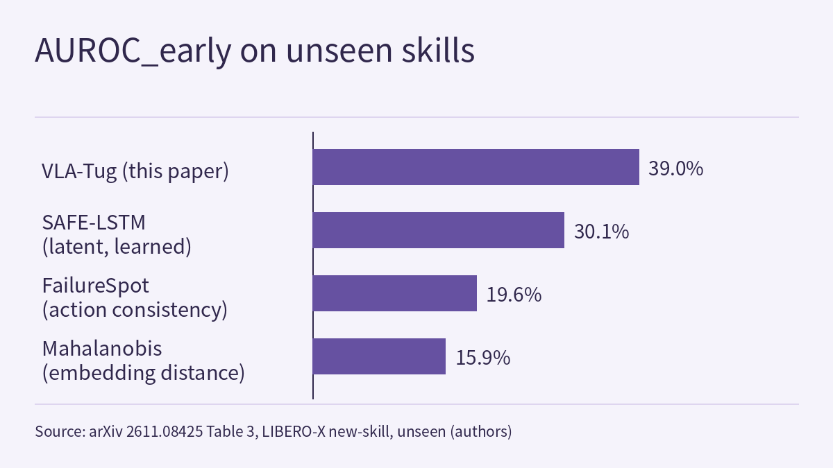
The metric is AUROC_early, defined by the authors: plot TPR_early (the share of failures with an alarm at or before t_fail) against FPR, take the area for FPR between 0 and 0.4, divide by 0.4 and express it as a percentage. Their reasoning is that a detector raising false alarms on more than 40% of successful rollouts cannot be deployed. Tasks are split into seen and unseen. The three LIBERO-X splits add distribution shift in turn: new-task holds out individual tasks, new-signature holds out a combination of components such as skill, target and relation, and new-skill holds out an entire skill. The table below is taken from the unseen-task columns of the paper’s Table 3 and lists 5 of its 9 methods, omitting STAC, ActProbe, Euclidean and PCA-KMeans; each cell is the mean over the splits of that setting:
| Method (type) | LIBERO-10 π0.5 | LIBERO-10 GR00T | LIBERO-X new-task | LIBERO-X new-signature | LIBERO-X new-skill | Real robot |
|---|---|---|---|---|---|---|
| VLA-Tug (this paper) | 47.9 | 47.4 | 40.2 | 47.0 | 39.0 | 25.8 |
| SAFE-LSTM (latent, learned) | 34.9 | 51.2 | 40.4 | 41.2 | 30.1 | 25.1 |
| SAFE-MLP (latent, learned) | 39.9 | 39.2 | 42.3 | 46.2 | 23.5 | 20.2 |
| FailureSpot (action consistency) | 36.2 | 44.7 | 20.4 | 26.2 | 19.6 | – |
| Mahalanobis (embedding distance) | 40.2 | 29.2 | 30.6 | 22.3 | 15.9 | 19.6 |
The abstract’s “up to 30%” corresponds to the new-skill column: 39.0 against SAFE-LSTM’s 30.1, which this site works out as about 1.30 times, an absolute difference of 8.9 percentage points. The authors report that the margin over SAFE-LSTM, the strongest learned baseline, grows with the shift: −1% on new-task, +14% on new-signature and +30% on new-skill. Two more things can be read from the table. VLA-Tug is the best method on new-signature, but its lead over SAFE-MLP there is only 0.8 points; on new-task the best method is SAFE-MLP. The authors themselves write that the lead on the real robot is small, that VLA-Tug does not lead on LIBERO-10 with GR00T, and that results on seen tasks are mixed. One more pattern stands out: Mahalanobis scores 85.7 on seen tasks of LIBERO-10 with π0.5 and drops to 40.2 on unseen tasks, so the gap between seen and unseen can be large. The table gives no spread across seeds.
Calibration: bound false alarms and missed detections together, or abstain
VLA-Tug picks its threshold with Learn-then-Test (LTT, Angelopoulos et al., 2022). The user sets an upper limit α on false alarms and a lower limit β on early detection. LTT tests each candidate threshold on the calibration set; with probability at least 1 − δ, every threshold it keeps satisfies both FPR ≤ α and TPR_early ≥ β, and it then selects the one with the highest TPR_early. The appendix states that both losses are binary, so p-values are exact binomial tails, with 181 candidate thresholds, multi-start fixed-sequence testing with 40 starts, and δ = 0.1. If no threshold passes, LTT abstains. The comparison methods, max-conformal (MC) and functional conformal (FC), both guarantee only the FPR, and the paper states that MC always returns a threshold.
The experiment uses 14 LIBERO-X runs (3 new-task seeds, 3 new-signature seeds and 8 new-skill folds) and 7 FPR targets from 10% to 50%, each paired with a TPR_early target. The authors report:
- On seen tasks, both LTT targets held in every certified run; MC met the FPR target in only 57–71% of runs.
- On unseen tasks, the FPR target held in 40–86% of certified runs, and the TPR_early target held in 57–90% of runs on unseen tasks (the wording of Section 6.2); MC reached at most 21% (the contribution list gives 0–21% for baselines).
- LTT abstained on 4–7 of the 14 runs, depending on the target (FPR targets of 15–50%). The authors read this as telling the user before deployment that the model cannot support the requested rates.
Watch the denominators. As this site reads it, “certified runs” exclude the 4–7 runs where LTT abstained, while MC never abstains, so 86% and 21% are not shares of the same set of runs. Abstention is useful information in itself, but it means that in those settings the system gets no usable threshold. The authors also state that on unseen tasks the samples are not exchangeable with the calibration set, so the guarantees hold only empirically, for all three methods; the shares come from 14 runs and are trends, not precise rates.
With a lower bound on TPR, one can give a conservative lower bound on the probability that an alarm means a real failure, the positive predictive value (PPV). From Bayes’ rule the paper derives PPV ≥ π·β / (π·β + (1 − π)·α), where π is the prior share of failures; the bound grows with π, so a lower estimate of π suffices. The authors report that this PPV lower bound is 58–71% across the FPR targets of their full table, held in every certified run on seen tasks and in 70–100% of runs on unseen tasks; the main text this site read does not say which value of π was used. A set of numbers assumed by this site shows how much π matters: with α = 0.1 and β = 0.8, π = 0.3 gives a lower bound of about 77%; if failures are rarer, π = 0.05, the bound is only about 30%. The same probe with the same threshold means something different depending on how common failures are where it is deployed.
Failure types, cost, and the steering demonstrations
Failure modes. The failure classes are strongly imbalanced, so the authors report balanced accuracy and compare against a majority baseline that always guesses the most common class (no existing baseline predicts failure modes). On LIBERO-X, top-1 accuracy improves over the majority baseline by up to 149% on seen and 79% on unseen tasks, and top-3 by a smaller but consistent margin; the abstract gives a top-3 gain on unseen tasks of up to 44%. On the real robot, top-1 improves by 171% and 8% on seen and unseen tasks. These are all relative gains; the main text this site read gives no absolute accuracies. The authors suggest narrowing a failure to three candidate classes and then choosing a stop, a retry or a handover to a human according to the riskiest of them.
Cost. The authors report: 6.8 s to train on one RTX 4090 (43.5 s for SAFE-LSTM); 6.6M parameters and 26.5 MB, about 0.2% of the VLA; under 2 ms per target pair on a CPU to calibrate. On LIBERO-X, each VLA call outputs 8 actions executed at 20 Hz, so a policy step lasts 400 ms; the probe adds 0.12 ms per step on the GPU (0.2% of a 54 ms GR00T policy call) and 0.9 ms on four CPU threads. For comparison, in Table 3 STAC takes 21.30 ms per step on the GPU, and the scoring state of Mahalanobis and Euclidean is 302.0 MB and 3056 MB.
Steering. The paper shows two examples. In simulation, for “place the largest bowl inside the left compartment of the bowl drainer”, the probe raises an alarm before the bowl goes into the right compartment; the end-effector is nudged to the left, the policy resumes and the rollout succeeds. On the real robot, for “put the mushroom in the plate”, the probe predicts an imminent grasp failure, the VLA is paused, an expert model shifts the trajectory to a successful one, and the VLA resumes. The correction tools in simulation are failure-mode-specific heuristics. The authors state plainly that the steering component is heuristic and not evaluated in the scope of the paper; the two examples are proofs of concept. For the abstract’s sentence about lightweight steering that improves task success, the main text gives no success-rate statistics.
How this relates to the course and earlier Radar items
Physical AI Lab 2.8: Reproducible Evaluation covers intervals for a binomial proportion and how to bound the failure rate after zero failures. LTT does the same kind of thing here: it treats “missed failures” and “false alarms on successes” in the calibration set as binomial counts and uses exact tail probabilities to decide whether a threshold can be certified. The difference is that LTT draws conclusions about two proportions at once and declines to give a threshold when the evidence is insufficient. Lesson 2.8 stresses that an interval describes only its own trials, criteria and setting; here that shows up directly as the exchangeability assumption: on unseen tasks, the guarantee keeps only an empirical meaning.
Physical AI Lab 1.8: Evaluation practised labelling failures. VLA-Tug’s conclusions depend on two kinds of labels, t_fail and the failure mode, and both are generated automatically by a video model; change how the labels are defined and both AUROC_early and TPR_early change with them.
Physical AI Lab 2.7: Safety Filters deals with another layer: a CBF filter sits on the fastest control loop and corrects actions step by step, with guarantees relative to the model. VLA-Tug runs at the pace of policy steps (400 ms per step here) and outputs “likely to fail, and probably which kind”; it decides when to pause or whom to hand over to, and it does not constrain actions directly. The two answer different questions, and one cannot replace the other.
RESETTLE, covered earlier on the Radar, triggers recovery when a frozen policy’s two action samples keep disagreeing, a signal of the kind the paper’s related-work and baseline sections call action consistency. VLA-Tug reads backbone embeddings instead, and makes threshold calibration and evaluation against failure time the focus of the paper.
Limitations
- This is an arXiv preprint; all numbers are reported by the authors [R], and this site has not reproduced them. The HTML text this site read is cut off at Appendix A.3, so the full calibration table and ablations in Appendix D were not read.
- Limitations listed by the authors: the calibration guarantees rely on exchangeability between calibration and test episodes, which weakens as distribution shift grows (empirically, they say, the degradation is gradual); the choice of backbone layer is not analysed systematically; the steering component is heuristic and not evaluated.
- 30%, 44%, 149% and similar figures are relative gains, and the denominator of 86% is certified runs, excluding abstentions. When quoting them, state the baseline, the setting and the denominator.
- Failure-time and failure-mode labels come from Gemini’s automatic annotation of videos, and the failure-time definition includes a judgement of when a human operator would take over.
- The main analysis is on layer 16 of GR00T-N1.7. The real robot covers only 8 tasks, and in the real-robot column only learned and embedding-distance methods have numbers.
- The abstract says the dataset is released on the authors’ project page, vla-tug.github.io; this site has not opened or checked that page or the dataset.
- None of these results is a hardware safety validation. A failure predictor provides the moment to pause or hand over; it does not replace safety constraints in the control layer or an emergency stop on site.
Links
- Failure Prediction and Classification in Vision-Language-Action Models via Calibrated Latent Probing (arXiv 2611.08425)
- Full paper in HTML
- Physical AI Lab 2.8: Reproducible Evaluation — Working Out Wald and Wilson Intervals by Hand, Sizing a Run from 1/√n, Then Bounding the Failure Rate after Zero Failures
- Physical AI Lab 1.8: Evaluation — Splitting a “Net Gain of 2” into a Paired Table, Then Checking the Failure Labels and Random Seeds
- Physical AI Lab 2.7: Safety Filters — Working Out One Control-Barrier-Function Correction by Hand, Then Choosing Its Loop and Its Safety Margin
- Frontier Radar | RESETTLE: step in only when a frozen policy’s two action samples keep disagreeing, then execute one demonstration-guided correction
- Physical AI Lab: a physical AI course where every number can be checked (course outline)