Lesson video
Narration is AI-generated. Video chapters, transcript and sources
Transcript
Transcript
UNIT-01 asks
Once a robot has learned a move, can it keep getting better on its own? This episode is about RL post-training. Letting a model learn from real trial and error, picking itself up after failure, and getting better and better.
From imitation to trial and error
First, imitation learning. Show the robot lots of demonstrations, and it copies them. But demonstrations rarely contain mistakes, or recoveries. Why does imitation get stuck? Demonstrations mostly cover the path where things go right. One slip takes it into states the demos never showed, so after getting something wrong it doesn't know what to do. Here's an example. Pouring coffee, the hand shakes, and it spills. A policy learned by imitation might just freeze right there. Reinforcement learning takes a different approach. Let the robot try for itself, and reward it when it does well. It learns to improve from its own experience. So the key word is post-training. Lay the foundation with demonstrations, then use trial and error to polish the policy, steady and fast. Foundation plus polish; you need both.
π*0.6 and RECAP
Let's look at a paper. It comes from Physical Intelligence. Their model is called pi-star zero point six. Their method is called RECAP. The paper says it uses advantage conditioning to bring reinforcement learning to VLAs. What does advantage conditioning mean? Put simply, it helps the model tell which action is better, and which is worse. Its data comes from three places. Human demonstrations, the robot's own runs, and people standing by, correcting it on the spot. Why human corrections? Because trying purely on its own is too slow, and too dangerous. With a helping hand, it learns faster and more safely. How well does it work? The paper says that on some of the hardest tasks, throughput more than doubled. And the failure rate was roughly cut in half. How real are these tasks? The paper says it can fold laundry in real homes. It can also assemble boxes, and make coffee with a professional machine. Another paper goes further. It does reinforcement learning directly on a real robot, with no simulation. Trying again and again, right in the real world. How long does training take? The paper says just one to two and a half hours, to reach a near-perfect success rate. How big is the improvement? The paper compares it with imitation learning baselines and prior RL methods. Its success rate is two times theirs on average, and execution about one point eight times faster. One of its secrets is a human in the loop. When the robot is about to make a mistake, a person lends a hand. Those corrections become learning signals too. So robots can learn from their mistakes too, and turn failure into skill!
The self-improvement loop
Put all this together, and you get a loop. See, think, act, get feedback, then update itself. The most important link in the loop is feedback. With good feedback, the policy knows which way to improve. Without it, it's just going in circles. Round after round, the policy climbs on its own. That's self-improvement. No need to teach it from scratch every time. You can train this way in simulation too. NVIDIA's Isaac Lab is an open-source framework. It supports reinforcement learning. How do you tell if RL helped? Do a before-and-after comparison. Measure the success rate, fine-tune with reinforcement learning, and see if it went up. Here is one training route. Train a teacher first, then distil it into a student. Finally, polish the student with reinforcement learning. The upside of simulation is massive parallelism, and nothing breaks. So trial and error can be fast and cheap. Real robots and simulation often work together. Get it mostly right in simulation, then fine-tune on the real robot. There's a trick in simulation called domain randomization. Randomly jiggle the lighting, friction, and mass. The policy becomes tougher. Another direction is fleet learning. Many robots work at once, pool their experience in one place, and grow stronger together. The more data, the more they've seen. Trial-and-error data is precious. Every real-robot run is slow and expensive. So every piece of experience has to be used to the full. Another trick is called curriculum learning. Start with easy tasks, then slowly make them harder. Don't jump straight to the hardest one. Trial and error on a real robot also needs safety. You need guardrails. Don't let it break itself, or its surroundings. Human corrections are great, but tiring. The ideal is this. The further along, the less a person has to step in. How to give rewards is a craft. Too sparse, and it can't learn. Too dense, and it easily learns the wrong thing. How do you confirm it really got stronger? Repeat the experiment and see how much the results vary. Don't be fooled by one lucky run: if the interval for the paired gain includes zero, all you can say is the evidence is insufficient. Back to the coffee example. After practice, when the hand shakes, it pauses. Steadies itself, then keeps pouring. Another approach is offline reinforcement learning. No more trial and error in real time. Instead, it learns again and again from stored experience. Why was this rarely done before? Because RL on real robots is hard to keep stable. One slip, and it diverges. So why does it work now? Because the algorithms are more stable. And because there's now a process for people to lend a hand. Let's be clear, though. Most of this is still one skill, on one robot. General-purpose is still a long way off. What's still unsolved is the cost. Reinforcement learning on real robots is slow, expensive, and may really break parts. Then there's how to set the reward. Once the reward is off, the robot will game it, and learn behaviour you never wanted. Even if it trains well in simulation, it may not adapt on a real robot. That's the old problem of going from simulation to reality. So the idea of post-training is imitation first, then trial and error. Let the policy keep growing from its own experience. The more it's used, the smoother it gets, and the better at recovering. Let's recap, three points. One, imitation sees few mistakes in the demos, so one slip and it gets stuck; RL learns recovery from trial and error. Two, RECAP brings RL to VLAs; the paper says that on some of the hardest tasks, throughput more than doubled and failures were roughly halved. Three, self-improvement is a loop, but real-robot RL is slow and expensive, and rewards are hard to set. Learn from others first, then practise on your own. Robots get stronger with every setback too! The policy is stronger now. But on long tasks, how does it remember, and how does it plan? See you next time!
Evidence and sources
Practice and self-check
The quiz is public and explains each answer as you go; answers to the guide's exercises are for signed-in members.
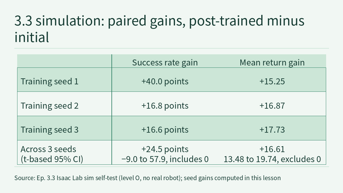
The video for episode 3.3 covers RL post-training: demonstrations mostly cover the path where things go right, so a policy learned by imitation easily gets stuck once it drifts away from them; reinforcement learning lets the policy learn recovery from its own experience, so you lay the foundation with demonstrations and then polish with trial and error. The video cites two papers: π*0.6 and RECAP from Physical Intelligence (arXiv 2511.14759), and HIL-SERL from UC Berkeley (arXiv 2410.21845); it also uses a simulation experiment the course ran itself in Isaac Lab to show how to confirm that a policy really got stronger. This page is the reading and exercises for the episode. It does not repeat the transcript; it does three things the video states as conclusions without working through. It puts HIL-SERL’s “1 to 2.5 hours”, “2x” and “1.8x” back with the system, baselines and task range the paper states. It uses a fictional workstation to show why “more than doubles task throughput” and “roughly halves the task failure rate” in the RECAP abstract are two different quantities. And it uses the per-seed numbers published in the experiment record to recompute, by hand, the paired 95% intervals for success rate and return, to see why the success rate can only be recorded as “insufficient evidence”. One rule runs through the whole page: a multiplier belongs only to the system, baseline and metric that produced it; with a different denominator, two multipliers cannot be converted into each other or combined into one conclusion.
The video, transcript and sources for this lesson are at the top of this page; the season plan is in the course outline. The previous lesson, Physical AI Lab 3.2: World Models — Making Data with Cosmos, Writing Down What Each Kind of Generation Is Conditioned On, Putting 78.3% Back in Its Human Evaluation, Then Setting Acceptance Rules for Generated Data, ended by asking how a trained policy can keep getting stronger through trial and error. This lesson picks up that question. How an error rolls out of the demonstrations’ coverage was worked out by hand in Physical AI Lab 1.6: Imitation Learning — Working Out How an Error Rolls Out of the Demonstrations’ Coverage, Then Putting the ACT, Diffusion Policy and Data Scaling Numbers Back in Their Own Conditions. How a return adds up and how a reward gets gamed was covered in Physical AI Lab 1.7: Reinforcement Learning — Working Out One Episode’s Return to See How a Reward Gets Gamed, Then Reading the Paper’s Terrain Curriculum and Time-out Resets. Parallel training in Isaac Lab was covered in Physical AI Lab 2.4: Parallel Walking Practice in Isaac Lab — Reading the Benchmark Table’s Three FPS Columns, Then Working Out a Run’s Total Steps from the Training Command. Domain randomization and sim2real were covered in Physical AI Lab 2.5: Sim2real with Domain Randomization and System Identification — Putting Two Papers’ Numbers Back in Their Setups, Then Working Out Friction by Hand from One Push of a Cup. Paired tables and Wilson intervals were worked out in Physical AI Lab 1.8: Evaluation — Splitting a “Net Gain of 2” into a Paired Table, Then Checking the Failure Labels and Random Seeds and Physical AI Lab 2.8: Reproducible Evaluation — Working Out Wald and Wilson Intervals by Hand, Sizing a Run from 1/√n, Then Bounding the Failure Rate after Zero Failures. This lesson does not repeat any of that; it covers what each of the three pieces of evidence for RL post-training measures, and how a t-interval across training seeds is computed. The full protocol and results of the experiment are in Physical AI Lab 3.3 experiment record: Isaac Lab simulation, 3 seeds (in Chinese). The site’s radar post Frontier Radar | Fine-tuning π0.5 on an SO-101 to move a chess king: cool down before comparing checkpoints, simulation pretraining helps most when real data is scarce, and training on own rollouts brings no measurable gain covers a different preprint, a different robot and a different setup; its results cannot be combined with the numbers in this lesson. The next episode, 3.4, covers long tasks: memory, planning and policy routing.
The public quiz’s 5 questions come with full explanations. Signed-in readers can do three exercises: recompute the paired 95% intervals from the experiment record’s per-seed numbers and estimate how many training seeds are needed; work out throughput, success rate and failure rate for a fictional coffee workstation and review four statements about multipliers; and review a fictional plan for real-robot RL post-training and rewrite it as a protocol that can be checked. Each comes with a step-by-step worked solution, common mistakes and a 20-point rubric.
1. HIL-SERL: the conditions attached to “1 to 2.5 hours” and “2x”
The HIL-SERL paper is an arXiv preprint by Jianlan Luo, Charles Xu, Jeffrey Wu and Sergey Levine of UC Berkeley. In this course’s grading it is level R; everything below is author-reported, and this site has not reproduced it. The two number cards in the video correspond to two sentences in the abstract, excerpted separately:
learn policies that achieve near-perfect success rates and fast cycle times within just 1 to 2.5 hours of training.
We show that our method significantly outperforms imitation learning baselines and prior RL approaches, with an average 2x improvement in success rate and 1.8x faster execution.
The introduction has one more sentence that states the conditions of the comparison with imitation learning:
Our trained RL policies greatly outperform imitation learning methods that are trained on the same amount of human data, e.g., same number of episodes of demonstrations or corrections, on average 101% improvement in terms of success rate and 1.8x faster in cycle time.
Four points matter when reading these numbers. First, “101% improvement” means 2.01 times the original, consistent with the abstract’s “2x”; the introduction states that the comparison is with imitation learning trained on the same amount of human data (the same number of episodes of demonstrations or corrections). The abstract also mentions prior RL approaches, and the passages read do not give separate numbers against them. Second, it is an average across tasks. Doubling a success rate is only possible when the baseline is at most 50%: for a task with a 70% baseline, double would be 140%, which cannot exist. So an average of 2x says nothing about how much any one task improved (this lesson’s arithmetic). Third, the introduction says “almost all of the tasks”:
However, perhaps the most surprising finding is that our system can train RL policies to achieve near-perfect success rates and super-human cycle times on almost all of the tasks with only one hour to 2.5 hours of training time in the real world.
Fourth, 1 to 2.5 hours is this system’s real-robot training time on these tasks. The passages read do not say whether it includes the time to collect demonstrations, train the reward classifier or set up the system.
The system is assembled from several parts, and the paper maps each to one difficulty: a pretrained visual backbone for optimization stability; a sample-efficient off-policy algorithm based on RLPD that also incorporates human demonstrations and corrections, for sample complexity; and a well-designed low-level controller to ensure safety during training. At each training step RLPD samples half of each batch from prior data and half from on-policy data. The reward is sparse:
For all our tasks, we employ a sparse reward function. This function makes a binary decision on whether a task is successful or not using a trained classifier.
Human corrections are data too:
During training, the system queries a human operator for potential corrections, which are then used to update the policy in an off-policy manner.
The paper says one difference from its predecessor SERL is that it uses both human demonstrations and corrections, while SERL uses demonstrations only; the authors consider adding corrections crucial for the policy to learn from its mistakes and improve, especially on tasks that are hard to learn from scratch. The tasks include whipping a Jenga block out of its tower, flipping an object in a pan, handing objects over between two arms, and assembling a motherboard, an IKEA shelf, a car dashboard and a timing belt, with one or two robot arms. The video warns that “most of this is still one skill, on one robot”. As this lesson reads it, every number belongs to these tasks, this hardware and this procedure; for another task, both the training time and the improvement have to be measured again.
Sign in to keep reading: the rest of this lesson, its self-check questions and the answers.
Limitations
- HIL-SERL and RECAP are both arXiv preprints at level R; the system structure, training times and multipliers are author-reported, and this site has not reproduced them or run any of the models. RECAP is Physical Intelligence’s report on its own model.
- For HIL-SERL this lesson read the abstract, the introduction, the related work and part of the start of Section 3; for RECAP only the abstract; for Isaac Lab only the documentation’s front page. The passages read do not give RECAP’s absolute values, which tasks count as “hardest”, the definition of throughput or the comparison, and do not say whether HIL-SERL’s training time includes preparation.
- The experiment record is the course’s own simulation experiment, level O, not a real-robot result; the reproduction scripts, raw logs and per-seed JSON are not public. Its initial policy is an under-trained PPO policy, and its conclusions cannot stand for RL post-training of VLAs.
- The following are this lesson’s summaries, arithmetic or inferences: 101% equals 2.01 times; a task with a baseline above 50% cannot double; the per-seed gains and the recomputed intervals; the reason for the 0.01 difference in the return interval; the evidence table and the recording checklist in section 4.
- The three responses and workstation B in section 2, and workstation K, team H, robot arm C, plan items P1–P5, the intervention counts and the seed gains in the transfer exercise, are all fictional and are not data from any paper or system.
- Paper calculations and simulation results are not hardware safety validation.
Links
- Physical AI Lab: a physical AI course where every number can be checked (course outline)
- Physical AI Lab 3.3 experiment record: Isaac Lab simulation, 3 seeds (in Chinese)
- Physical AI Lab 3.2: World Models — Making Data with Cosmos, Writing Down What Each Kind of Generation Is Conditioned On, Putting 78.3% Back in Its Human Evaluation, Then Setting Acceptance Rules for Generated Data
- Physical AI Lab 1.6: Imitation Learning — Working Out How an Error Rolls Out of the Demonstrations’ Coverage, Then Putting the ACT, Diffusion Policy and Data Scaling Numbers Back in Their Own Conditions
- Physical AI Lab 1.7: Reinforcement Learning — Working Out One Episode’s Return to See How a Reward Gets Gamed, Then Reading the Paper’s Terrain Curriculum and Time-out Resets
- Physical AI Lab 1.8: Evaluation — Splitting a “Net Gain of 2” into a Paired Table, Then Checking the Failure Labels and Random Seeds
- Physical AI Lab 2.4: Parallel Walking Practice in Isaac Lab — Reading the Benchmark Table’s Three FPS Columns, Then Working Out a Run’s Total Steps from the Training Command
- Physical AI Lab 2.5: Sim2real with Domain Randomization and System Identification — Putting Two Papers’ Numbers Back in Their Setups, Then Working Out Friction by Hand from One Push of a Cup
- Physical AI Lab 2.8: Reproducible Evaluation — Working Out Wald and Wilson Intervals by Hand, Sizing a Run from 1/√n, Then Bounding the Failure Rate after Zero Failures
- Frontier Radar | Fine-tuning π0.5 on an SO-101 to move a chess king: cool down before comparing checkpoints, simulation pretraining helps most when real data is scarce, and training on own rollouts brings no measurable gain
- Luo et al.: Precise and Dexterous Robotic Manipulation via Human-in-the-Loop Reinforcement Learning (HIL-SERL, arXiv 2410.21845)
- Physical Intelligence: π*0.6 and RECAP (arXiv 2511.14759)
- NVIDIA Isaac Lab documentation