The preprint VLA Adaptation with Real and Simulated Data: A Case Study on Robotic Chess (arXiv 2611.12676, 2026-11-09, Matěj Kripner and Milan Straka, Faculty of Mathematics and Physics, Charles University, Prague) uses one narrow task to answer practical questions that come up when fine-tuning a VLA: how many demonstrations to collect, how long to train, which checkpoint to deploy, and whether simulated data is worth using. A low-cost SO-101 arm moves a chess king on instructions such as “Move the king from e4 to a5”, and the model is π0.5. The authors report four findings. Checkpoints must be compared after the learning rate has been cooled to zero, otherwise results from the same run differ by up to 31 points. Validation loss and offline action error do not pick good models. When real demonstrations are scarce, pretraining on simulated demonstrations helps most. Further training on the policy’s own rollouts brought no measurable improvement. All numbers below are author-reported [R]; this site has not reproduced them.
Task, arm and simulated twin
The instruction names only the source and target squares. The policy has to find both squares on the board it sees, then grasp, carry and place the king, and return to the ready pose. The board is wooden with 31 mm squares; the king is 64 mm tall on a 20 mm base. The authors list why the task is hard for the SO-101: squares can only be located from their names; the arm’s posture changes a lot, from steeply folded near the base to almost fully extended at the far ranks; the gripper has one fixed finger and one moving jaw, so a grasp a few millimeters off the king’s axis topples it; and the 3D-printed links flex by up to 2 cm under load, so the arm cannot be positioned precisely without visual feedback.
The real setup has two cameras, one on the wrist looking along the gripper and one fixed above the board. Both have fisheye lenses, and their images are rectified to the simulator’s pinhole model before the policy sees them. The simulator is a MuJoCo twin of the real setup. It reproduces the arm’s kinematics and servo dynamics, the measured board pose, the scanned king, and the poses and fields of view of both cameras, but it does not model the compliance of the printed links.
Simulated demonstrations come from a randomized scripted expert. The authors’ reasoning is that a motion planner would execute every move identically, which neither resembles teleoperation nor gives imitation learning enough variation. The expert therefore imitates a human operator: it reaches for a target with a perception error, observes the remaining error after a latency and corrects, until the error is below a tolerance. Each episode samples its own tempo, errors, tolerances and grasp parameters, and the expert reopens and retries after a missed grasp. It succeeds in 93% of its episodes.
The policy starts from π0.5, which was not pretrained on the SO-101. It receives the two camera views, six joint positions, the instruction and the current stage, and outputs chunks of 50 joint targets at 15 Hz, executing 10 of them before planning again. The authors fine-tune the action expert and the language model, 2.7B of the model’s 4.1B parameters, and keep the vision encoder frozen. The language model also predicts, as one token, which of the five stages of a move the arm is in. At test time the policy re-scores the current and next stage once per action chunk and advances when the next stage wins twice in a row.
Scaling in simulation: enough data and enough updates
The simulated set holds about 11.4k expert episodes with the king offset by up to 8 mm inside its square, 93% of them successes. Training sets are nested subsets of the successes with n = 100, 316, 1,000, 3.2k and 10k, plus 30 held-out successes for validation. Every run uses a constant learning rate of 3 × 10⁻⁵ after 500 warm-up steps and a global batch of 32 frames. Update budgets form a geometric ladder of 8 steps from 1,000 to 165k (one epoch of the largest set), extended to 237k for the two largest sets. Each configuration is trained once. Each model runs 1,000 closed-loop trials on a fixed schedule of moves, and success rates carry Wilson 95% intervals of about ±3 points at 30–60% success.
The results read along two axes:
- Below about 4k updates no model succeeds, whatever the dataset size.
- At small update budgets, more data barely helps: at 9k updates, 1,000 and 10k demonstrations give 10% and 11%.
- In the authors’ grid, a smaller dataset performs as well as a larger one until its first epoch is complete and falls behind afterwards. Training for many epochs still helps and never lowers success beyond the evaluation noise.
- At 165k updates (all cooled down), the five dataset sizes reach 9.9%, 22.0%, 31.7%, 39.7% and 60.2%. With 10k demonstrations, training to 237k updates gives 64.1%, and success is still rising.
Two comparisons cover only the 10k-demonstration size. Without π0.5’s robot pretraining (vision-language model initialized from PaliGemma, action expert initialized randomly), the model also reaches 59.5%. Fine-tuned with their stock recipes, π0 reaches 77.7% and SmolVLA 54.5%. The authors note that those recipes differ from theirs, so these numbers compare model and recipe together, and that robot pretraining may still matter with smaller datasets.
Choosing a checkpoint: cool down first, ignore offline metrics
For each dataset size the authors run one constant-rate trunk, keep a checkpoint at 90% of each budget, and branch from it to cool the learning rate to zero over the remaining 10% of updates. With 10k demonstrations, the branch ending at 165k updates reaches 60%, while the constant-rate checkpoint it started from reaches 29%; that gap is the “up to 31 points” in the abstract. The trunk’s own checkpoint at 165k updates reaches 49%. The trunk’s success is not monotonic in the number of updates, and early stopping on its checkpoints would select a model 18 points below what the run reaches with a cool-down. Initial results suggest stochastic weight averaging (SWA) over the same updates is nearly as effective: 57% against 60% for the cool-down.
The offline metrics fail more plainly. With 100 demonstrations, validation loss is lowest at about 2k updates and more than doubles by the end of training, while success rises from 0 to 10%; selecting by validation loss would return a model with zero success. Open-loop action error does fall monotonically, but it does not separate models: at about 79k updates it is 22–24 mm for all five dataset sizes, while the cooled-down models range from 8% to 48% success.
By milestone, most failures after a grip are toppled kings, in about a third of all trials, and the cool-down mostly improves grasping and placing. In their conclusion the authors write that, in their setting, fine-tuning choices could only be judged by closed-loop evaluation on many trials, which the simulator made affordable. Physical AI Lab 2.3 covers preparing demonstrations for fine-tuning SmolVLA and checking what each number measures. This paper adds the step after training: which checkpoint to deploy, and why a loss curve alone cannot decide it.
Real arm: simulation pretraining matters most when real data is scarce
One of the authors teleoperated 261 king moves with the leader arm. Source and target squares were drawn at random, and the king was placed up to 8 mm off the center of its square, as in the simulated data. 259 of the moves are successes and form the real dataset, about half an hour of motion in total. Fine-tuning starts from two initializations: the released π0.5 itself (base-initialized below), and the simulation model trained on 10k simulated demonstrations for 237k updates and cooled down, with 64% success in simulation (sim-initialized below). Real data comes in nested random subsets of 32, 128 and 256 demonstrations, with the same recipe as in simulation: a trunk to 45k updates with checkpoints at 90% of the 2k, 15k and 45k budgets, each cooled down, and the trunk extended to 75k updates for one more cooled-down model.
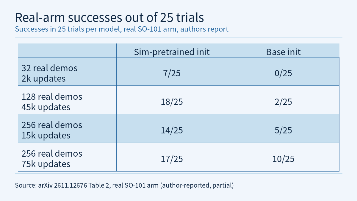
Every model runs the same 25 trials, the first 25 moves of the simulator’s easy schedule, with the king centered on its square. The policy runs autonomously at one third of the demonstrated tempo because of inference latency in the deployment. A trial that exceeds 60 s of control time counts as a failure, and failed trials are never discarded. The evaluator only resets the king and grades the highest milestone reached. The results are partial: ten models in five pairs (Table 2 of the paper; each cell is a count out of 25):
| Real demos | Updates | Sim-pretrained: touched | Gripped | Success | Base: touched | Gripped | Success |
|---|---|---|---|---|---|---|---|
| 32 | 2k | 25 | 12 | 7 | 6 | 0 | 0 |
| 128 | 45k | 25 | 24 | 18 | 15 | 8 | 2 |
| 256 | 15k | 25 | 23 | 14 | 23 | 13 | 5 |
| 256 | 45k | 25 | 22 | 14 | 23 | 17 | 10 |
| 256 | 75k | 25 | 23 | 17 | 24 | 15 | 10 |
The sim-initialized policy is better in all five pairs. With 128 demonstrations it succeeds in 18/25 trials against 2/25. With 32 demonstrations the sim-initialized policy succeeds in 7/25, while the base-initialized policy never grips the king, 0/25. With 256 demonstrations the gap is smaller: 14/25 to 17/25 for sim-initialized and 5/25 to 10/25 for base-initialized. The authors state that with 25 trials per model they only interpret large differences. Physical AI Lab 2.8 shows how to compute Wilson intervals for success rates of this size, which helps judge which differences in the table hold up.
Of the gaps between simulation and the real arm, the authors handle two. Fisheye frames are rectified to the simulator’s intrinsics in both training and deployment, and the constant per-joint offset between the real calibration’s joint zeros and the simulator’s is absorbed by normalizing with the real dataset’s statistics. Two gaps are not handled: the real policy runs at a third of the demonstrated tempo, and the simulator applies the 15 Hz joint targets as steps where the real controller interpolates them. In addition, the recorded frame rate varied between 15 and 23 frames per second across sessions and was stored as 30, so the policies were trained on a mix of apparent tempos. Physical AI Lab 2.5 covers domain randomization and system identification for sim2real; this paper gives a concrete list of which gaps were corrected and which were left alone, and simulation pretraining still improved results on the real arm.
A negative result: training on the policy’s own rollouts
In simulation, the authors test whether the policy improves from its own rollouts. They take the best behavior-cloning model for a dataset size (165k updates), run it on new moves from the collection distribution, record every trial with its graded outcome, and train a new policy from the base model on demonstrations plus rollouts. There are two rounds. 1K+1K uses 1,000 demonstrations plus 1,000 rollouts of a model with 32% success; 10K+10K uses 10k demonstrations plus 10k rollouts of a model with 60% success. The baseline is behavior cloning on the demonstrations alone for the same number of updates.
- Filtered BC (adding only successful rollouts): in 1K+1K, 33% against 30% for behavior cloning at 79k updates, and 34% against 32% at 165k. It is about three points ahead at two intermediate budgets, but not at the largest one.
- RECAP-style advantage conditioning (labels from a value function, from a cross-fitted value function, or from outcomes): 30–31% at 79k updates, matching behavior cloning. The policy does use the label: the outcome-label model reaches 30% sampled with the positive label, 26% with no label and 24% with the negative label. Classifier-free guidance at β = 1.5 gives 31%, and β = 2.5 lowers it to 23%. In the 10K+10K round, outcome labels reach 46% at 79k updates against 48% for behavior cloning.
- Value function: a large value function on the policy’s 3B backbone, trained for two epochs, memorized its training episodes and was at chance on unseen ones. The authors switched to a smaller value function trained for one epoch; on held-out episodes it separates successes from failures with an AUC of 0.85 four seconds into the episode, before the grasp.
- Corrections from an automatic coach: in the original RECAP a person corrects the policy during rollouts. The authors replace that with a monitor in simulation that hands control to the scripted expert when the king tilts or slides, when a grasp misses, or when a forward simulation predicts a topple, and returns control after the fix. Trained on about 1,000 coached rollouts, coached RECAP reaches 35% on the hard schedule, above behavior cloning at 30% (paired McNemar test, p < 0.02), but 46% against 50% on the easy schedule.
- Residual reinforcement learning: a small network trained with PPO from privileged simulator state adds a joint offset of at most 3° to the frozen policy’s actions. Across four runs with different rewards and exploration noise, success stayed within evaluation noise of its initial value.
The authors conclude that, in their setting, none of these methods gave a measurable improvement over plain behavior cloning, and the failed rollouts, which only the labeled variants see, gave no measurable benefit. Their limitations section states that these RECAP variants omit the original’s advantage-conditioned pretraining and human corrections, so the negative result applies to the versions they implemented.
Limitations
- This is an arXiv preprint. All numbers are author-reported [R]; this site has not reproduced them or run the released simulator or data.
- There is one task, and each setting is trained once, so there is no variance across training seeds.
- Real-arm evidence is limited: 25 trials per model and ten models evaluated, which the authors themselves call partial. In the real evaluation the king starts centered on its square, while the training data places it up to 8 mm off center, so the evaluation does not cover offset placements.
- The scripted expert is randomized, but its similarity to human demonstrations is not rigorously measured. The paper only describes the human operator’s paths as showing a similar spread, with straighter carries.
- The π0, SmolVLA and no-robot-pretraining comparisons in simulation cover only 10k demonstrations and cannot be extended to smaller datasets.
- All success rates measure task completion and involve no safety validation of the arm’s motion; simulation results are not a real-arm or safety validation.
Links
- VLA Adaptation with Real and Simulated Data: A Case Study on Robotic Chess (arXiv 2611.12676)
- Full paper in HTML
- Code repository given in the paper: kripner/vla-chess (simulator and scripted expert)
- Real demonstration dataset given in the paper (LeRobot format, 261 episodes)
- Physical AI Lab 2.3: Fine-Tuning SmolVLA — Planning Demonstrations for an Instruction, Checking What Each Number Measures, Then Timing the Asynchronous Action Queue
- Physical AI Lab 2.5: Sim2real with Domain Randomization and System Identification — Putting Two Papers’ Numbers Back in Their Setups, Then Working Out Friction by Hand from One Push of a Cup
- Physical AI Lab 2.8: Reproducible Evaluation — Working Out Wald and Wilson Intervals by Hand, Sizing a Run from 1/√n, Then Bounding the Failure Rate after Zero Failures