A world-action model (WAM) predicts future frames while it generates robot actions. The future video is denoised step by step, so inference is expensive. Most existing speed-ups give future refinement a fixed budget, whatever the current task and execution state. In the preprint Elastic-WAM (arXiv 2611.14257, 2026-11-10), Haitian Li and colleagues at the National University of Singapore, RoboScience and other institutions let a learned “refinement demand field” make three decisions per state: when to stop refining the future video, how far the next denoising step advances, and which future video tokens to refresh. The base WAM stays frozen throughout. The authors report a mean success rate of 57.4% on RoboCasa-GR1 at an inference latency of 388.2 ms, 32.2% below Joint-WAM (572.6 ms), which uses the same backbone. All numbers below are reported by the authors [R]; this site has not run their code.
Method: one refinement demand field, three decisions
The authors first looked at 10 selected tasks from LIBERO-Plus. The number of denoising steps that gave the highest success rate ranged from 1 to 4 across tasks, and within a single task different states preferred different refinement depths. Action-to-video attention maps also showed that action generation attends unevenly to different regions of the future frames. From this the paper argues that refinement compute should be allocated on demand along two axes: denoising time and future video space.
Concretely, the 196 future video tokens are split into 64 groups that keep temporal and camera-view boundaries, each with 1, 2 or 4 tokens. Each group has a “remaining demand” curve over normalized denoising progress z ∈ [0, 1], written as an amplitude times a Beta density. Because all future tokens follow the same denoising trajectory in the base WAM, the authors let the groups share one temporal basis B0 and vary only the amplitude: each group’s amplitude is sigmoid(b0 + Δu_g), where b0 is a global offset and Δu_g is a relative score centred by its token-weighted mean. The token-weighted mean of all group amplitudes gives the total remaining demand D(s). With this split, the global offset only governs how much refinement is left, and the relative scores only govern where to refine first. The three decisions are read from the field:
- When to stop (WHEN): D at each step is treated as the conditional probability of continuing, and the cumulative “World Commit” probability is 1 minus the running product of the per-step D. Refinement of the future video stops once that cumulative probability reaches 0.5.
- How far to go (HOW FAR): taking the mode z_k of the shared temporal basis, the next noise reduction is δmin + z_k(δmax − δmin), with δmin = 0.05 and δmax = min(0.20, σ_k − σ_floor).
- Where to refresh (WHERE): under a budget of exactly K0 tokens, the groups with the highest relative scores are selected; by default each sparse update refreshes K0 = 96 tokens. The budget is set externally, and the learned scores only decide which regions are chosen.
Training and inference: the WAM is frozen, only the field is learned
The backbone is FastWAM-Joint. The paper states that this is the model the Faster-WAM paper calls Joint-WAM, so Joint-WAM in the comparison tables is the same backbone without this mechanism. Training has three stages; each learns one part of the parameters with the rest frozen:
- Temporal profile: from the same recurrent state, an “immediate commit” is compared with “one more step” at several denoising distances. Each candidate runs action denoising to the end and is scored by the terminal action error E = 0.6 E_seq + 0.4 E_Δ (action-sequence error and the error in consecutive action differences). Candidates with lower error get higher probability in a soft target that supervises B0; the same comparisons also train a temporal teacher that judges when to stop.
- Spatial priorities: at the same denoising state, a dense update without gradients serves as the teacher and a differentiable sparse update as the student; gradients for the discrete fixed-budget mask come from a straight-through approximation. Gradients pass through the frozen WAM’s computation and update only the spatial scores.
- Overall demand: the temporal teacher’s stopping predictions give a target continuation probability for each step, which is converted to a target global offset b0. Training runs on complete recurrent prefixes and constrains the cumulative stopping probability and the commit timing.
At inference, each replanning cycle starts with one dense joint denoising step over all future tokens, which sets up the recurrent state and the layer-wise key–value cache. At each later step the observation and action queries stay dense, and only the selected future video queries are recomputed, still with access to the full logical key–value context. Unselected tokens keep their cached hidden states, keys, values and the velocities from their last refresh. When the cumulative commit probability reaches the threshold, or when what the paper calls a “safety condition” is triggered, refinement of the future video stops and action denoising continues directly from the current video representation and cache, with no further video prefill. The text read does not say what this safety condition is.
Simulation results and latency
The four simulation benchmarks are LIBERO (4 suites, 50 rollouts per task, 2,000 episodes in total), LIBERO-Plus (7 perturbation categories), LIBERO-Pro (4 categories of generalization changes) and RoboCasa-GR1 (24 tasks, following StarVLA’s evaluation setting). On LIBERO-Plus and LIBERO-Pro the LIBERO-trained policy is evaluated without further adaptation. Mean success rates (%):
- LIBERO: Elastic-WAM 98.8, Joint-WAM 98.5, LingBot-VA 98.5, π0.5 96.9. The authors stress the gain over Joint-WAM on the Long suite (98.2 vs 96.8), but LingBot-VA scores 98.5 on that suite.
- LIBERO-Pro: Elastic-WAM 54.1, π0.5 53.4, Joint-WAM 52.8. Of the four categories, Position is low for every method: 8.4 for Elastic-WAM, 20.8 for π0.5.
- LIBERO-Plus: Elastic-WAM 73.7, OpenVLA-OFT 69.6, LingBot-VA 69.5, Joint-WAM 66.3, Fast-WAM 49.1.
The paper’s text says Elastic-WAM is more robust across all LIBERO-Plus perturbation categories. By the paper’s own Table 3, this holds against Joint-WAM, which it beats in all seven categories, but not against the other baselines. In four categories at least one baseline scores higher: camera viewpoint, π0-Fast 65.1 and OpenVLA-OFT 56.4 vs Elastic-WAM’s 52.1; robot initialization, LingBot-VA 83.0 vs 76.3; background, OpenVLA-OFT 93.3, π0 81.4, UniVLA 81.0 and π0-Fast 73.2 vs 60.0; sensor noise, π0 79.0, OpenVLA-OFT 75.8, π0-Fast 74.4 and LingBot-VA 64.4 vs 61.1. The paper names camera viewpoint, robot initialization and sensor noise as its “particularly notable gains”; all three are among these four categories. The introduction also limits the abstract’s “state-of-the-art” to “among methods without large-scale embodied pretraining”.
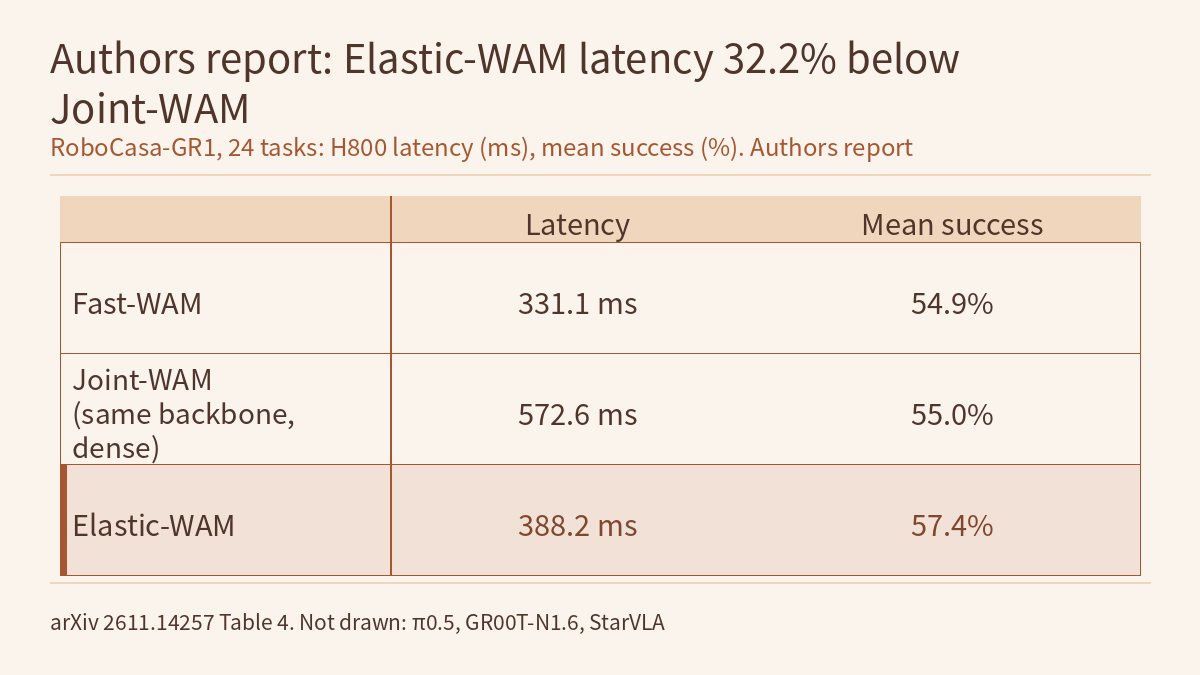
Latency is reported only on RoboCasa-GR1, in ms, measured on one NVIDIA H800 GPU. The three WAM rows of the paper’s Table 4:
| Method | Inference latency (ms) | Mean success (%) |
|---|---|---|
| Fast-WAM | 331.1 | 54.9 |
| Joint-WAM | 572.6 | 55.0 |
| Elastic-WAM | 388.2 | 57.4 |
The 32.2% is the reduction relative to Joint-WAM, (572.6 − 388.2) / 572.6. Fast-WAM drops explicit future video generation at inference; its latency is 57.1 ms lower than Elastic-WAM’s, and its success rate 2.5 percentage points lower. The three VLA baselines in the same table, π0.5, GR00T-N1.6 and StarVLA, run at 77.0–82.0 ms with success rates of 37.0–48.8%; Elastic-WAM’s latency is about 4.7–5.0 times theirs (this site’s calculation from the table). The text read does not say what one latency measurement covers, for example whether it is one replanning cycle, and gives neither the action-chunk length nor the control rate.
Ablations and the real-robot trials
All ablations use the frozen backbone. Each cell gives one success rate; the paper does not state the number of runs or seeds:
- Spatial selection (RoboCasa-GR1, Table 5): learned selection with 96 tokens per step gives 57.42%; random selection with the same budget 53.83%; all-active with K = 128 55.17%; FirstKV, which follows Faster-WAM in reusing the initial video cache without further refinement, 54.50%.
- Temporal control (LIBERO-Plus, Table 6a, spatial selection and budget fixed): spatial selection only 71.71%, adding adaptive commit with a fixed step size 72.31%, adaptive commit and step size 73.71%.
- Refresh budget (LIBERO-Plus, Table 6b): K = 49 gives 72.84%, K = 96 73.71%, K = 147 71.71%, and K = 196 (all 196 future tokens) 70.92%. The authors conclude that refreshing more future tokens does not necessarily improve downstream control.
The real-robot trials use a bimanual platform of two UFACTORY xArm 7 arms on a four-stage tea task: place the white cup on the uncovered teapot, pour tea from the covered teapot into the white cup, return the white cup to its place, then pour tea from the uncovered teapot into the black cup and return the teapot. The authors collected 200 demonstrations and ran 20 trials per method under each of three conditions: nominal, neon lighting (Lighting OOD), and the white cup replaced by a silver cup of slightly different shape (Object OOD). SR is the share of trials that complete all four stages; PS is the mean fraction of the four stages completed.
- Elastic-WAM: SR 50.0 / 50.0 / 30.0, PS 57.5 / 52.5 / 47.5.
- Joint-WAM: SR 30.0 / 30.0 / 30.0, PS 37.5 / 35.0 / 35.0.
- Fast-WAM: SR 0.0 under all three conditions, PS 12.5 / 5.0 / 10.0.
In trial counts, 50.0% is 10 of 20 and 30.0% is 6. The real-robot section reports no latency. The authors explain the long-horizon advantage as a hypothesis: adapting temporal progression and spatial allocation together may help the policy tell from visual changes which stage it is in. They say this is consistent with the LIBERO Long suite and the real-robot PS results; the text read contains no experiment that tests this mechanism directly.
How to read these numbers
What is new in this paper is compute allocation: it leaves the base WAM unchanged and decides, per state, how much of the future video to refine and where. Forward Dynamics Models, covered earlier on this site, takes a different route and skips future generation at inference; HWAM also used Fast-WAM as a baseline. For what a world model predicts and what it is conditioned on, see Physical AI Lab 3.2.
Three points matter when reading the latency. First, the 32.2% compares against dense refinement on the same backbone, not against the fastest method; Fast-WAM is faster, and the VLA baselines are much faster. Second, 388.2 ms is an H800 figure and will differ on onboard hardware. Third, the control rate one inference can sustain depends on how many action steps each inference executes, which the paper does not give; how to work out a control-rate ceiling from latency is covered in Physical AI Lab 2.6.
For the success rates, no table in the paper reports a confidence interval, random seeds or repeat counts. Several simulation gaps are only 1 to 3 percentage points, such as 57.4 vs 55.0 on RoboCasa-GR1 (a gap of 2.4 percentage points) and 73.71 vs 72.31 in the ablation. The real-robot runs have only 20 trials per condition. A rough Wilson calculation by this site gives a 95% interval of about 29.9%–70.1% for 10/20 and 14.5%–51.9% for 6/20, which overlap widely. The hand calculation is in Physical AI Lab 2.8, and paired comparison in Physical AI Lab 1.8. PS is higher than Joint-WAM’s under all three conditions, a consistent direction, but again without intervals.
Limitations
- This is an arXiv preprint; all numbers are reported by the authors [R], and this site has not reproduced them. The text read does not say whether code or weights are released.
- No table reports intervals or seeds, so neither the 1–3 point gaps in simulation nor the gaps over 20 real trials should be read as a firm ordering.
- Latency is measured only on RoboCasa-GR1 on a single H800; the real-robot trials report no latency and no control rate.
- The paper says Elastic-WAM is more robust in every LIBERO-Plus category; by its Table 3 this holds only against Joint-WAM.
- The number of tokens refreshed per sparse update, K0 = 96, is an externally set hyperparameter, not a learned one. It scores highest on LIBERO-Plus in Table 6b, and the paper does not say whether the default was chosen on that same evaluation.
- The “safety condition” that stops refinement is not defined in the text read. The real-robot trials cover one task under three conditions and are not a hardware safety validation.
Links
- Elastic-WAM: Adaptive Spatiotemporal Imagination for Efficient Robot Control (arXiv 2611.14257)
- Full paper in HTML
- Frontier Radar | Forward Dynamics Models: future prediction reads action features, actions never read the future, and inference skips future generation
- Frontier Radar | HWAM: a humanoid’s reference action is not the motion it performs, so generate the post-execution body state alongside it
- Physical AI Lab 3.2: World Models — Making Data with Cosmos, Writing Down What Each Kind of Generation Is Conditioned On, Putting 78.3% Back in Its Human Evaluation, Then Setting Acceptance Rules for Generated Data
- Physical AI Lab 2.6: To the Edge — Working Out the Control-Rate Ceiling from a Latency Log, Telling Whether Quantization Saves Size or Time, Then Sizing an Action Chunk
- Physical AI Lab 2.8: Reproducible Evaluation — Working Out Wald and Wilson Intervals by Hand, Sizing a Run from 1/√n, Then Bounding the Failure Rate after Zero Failures
- Physical AI Lab 1.8: Evaluation — Splitting a “Net Gain of 2” into a Paired Table, Then Checking the Failure Labels and Random Seeds
- Physical AI Lab: a physical AI course where every number can be checked