The preprint DEED (arXiv 2610.40430, 2026-10-29, Jingxu Gu and Dongze Lian, Nanjing University) is a report on a competition entry: adapting the pretrained VLA Xiaomi-Robotics-1 to the five simulated fine-grained manipulation tasks of MetaFine. It proposes no new model architecture. It changes two things: how the demonstrations fed to the model are distributed, and how the model’s predicted action chunks become robot commands. The authors report an official Overall score of 85.55%, against 43.01% for the π0 baseline published on the same leaderboard. The more useful part is the breakdown: two of the five tasks score only about 64.6%, and several fixed-policy comparisons show that deployment settings such as execution horizon, denoising steps and gripper mapping visibly change the results. All numbers below are author-reported [R]; this site has not reproduced them.
What MetaFine tests, and what plain fine-tuning misses
As the paper describes it, MetaFine tests fine-grained manipulation with five tasks: part-level grasping, directional motion, switch toggling, object sorting and letter insertion. Going by the instructions in the paper’s Table 1, these are T1 (the part cap or body), T2 (forward, left, right), T3 (red or blue switch), T4 (red, blue, green cube) and T5 (letters C, o, R, L). Evaluation has three dimensions: Perception (P, perception under camera and illumination changes, scored as AUSC, the area under the success curve), Understanding (U, instruction-conditioned behavior) and Controlled Behavior (B, controlled behavior during execution). Each task score is the mean of P, U and B, and Overall is the mean of the five task scores.
The authors argue that fine-tuning a pretrained VLA directly on the provided demonstrations leaves three gaps:
- Scene and instruction are confounded. If different instructions only ever appear in different scenes, a policy can pick its target by recognizing the scene rather than reading the instruction. Inspecting the released T5 metadata, the authors found disjoint scene seeds across letter subsets, which opens the way to this shortcut.
- Visual coverage is too thin. The demonstrations contain too few camera positions and lighting conditions.
- The execution interface does not match. Predicted action chunks can fail when the execution horizon, the inverse-kinematics conversion or the gripper semantics do not match the simulator interface.
Demonstration expansion: new instructions for the same scene, new images for the same trajectory
Instruction pairing. For one initial scene, the official expert planner generates a trajectory for each instruction in that scene’s instruction family: the initial layout is shared, while the target and the following motion depend on the instruction. A generated family is kept only when every instruction variant succeeds. The same initial image then leads to different decisions, so the only way for the policy to tell them apart is to read the instruction.
Re-rendering from physical states. In the benchmark’s own ManiSkill3/SAPIEN simulator, each state of a saved trajectory is restored and the base-camera and hand-camera images are rendered again under new camera and lighting parameters. Proprioceptive input and future action targets stay unchanged and remain tied to the original physical states. The paper stresses that only observation formation changes, so viewpoint-dependent geometry and action labels stay aligned. Perturbations come in three levels: camera translation bounds of 0.03, 0.06 and 0.12 m and rotation bounds of 2°, 6° and 12°; lighting half-widths of 0.10, 0.25 and 0.40 around ambient RGB 0.5. All five tasks use camera and lighting perturbations; only T5 also uses combined camera-and-lighting perturbations, and combined rendering covers 120 base trajectories.
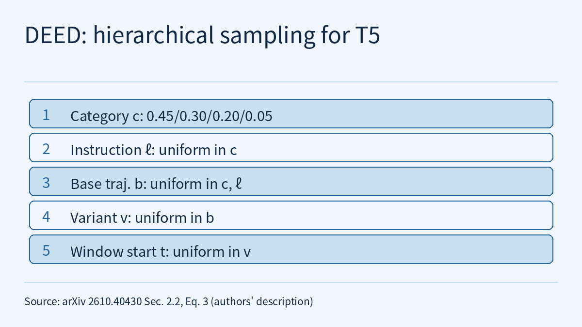
Hierarchical sampling. After expansion, trajectories with many rendered copies would be drawn more often. The T5 data loader therefore samples level by level: first an augmentation category with prescribed probabilities (clean, camera, lighting and combined at 0.45, 0.30, 0.20 and 0.05), then an instruction uniformly within that category, then a base trajectory uniformly, then a rendered variant of that trajectory uniformly, and finally a training-window start uniformly. Because base trajectories are drawn before rendered variants, extra rendered copies do not raise a trajectory’s chance of being drawn within a category and instruction. The paper notes explicitly that this probability is the training-data sampling distribution, not the policy’s action probability.
The final T5 pool holds 2,800 distinct successful trajectories and 7,840 records after rendering, including 2,000 new motions generated from 500 four-instruction scenes. Record counts (including rendered variants) for the other tasks are T1 6,400, T2 3,300, T3 2,080 and T4 2,940.
The model inputs are the task instruction, base and hand-eye RGB images, and joint and gripper state (seven arm joint positions plus the mean of the two finger positions). It predicts K = 30 end-effector actions at a time, generated with flow matching. The authors keep Xiaomi-Robotics-1’s architecture and released training implementation. The final T5 continuation used 12,000 BF16 updates (batch 4), a cosine learning-rate schedule from 3 × 10⁻⁶ to 5 × 10⁻⁷, and 300 warmup updates.
Execution design: how an action chunk becomes joint commands
At deployment, the policy’s local end-effector offsets are converted into world-frame targets and then into seven joint increments by inverse kinematics. Finger targets are clipped to the range −0.01 to 0.04 m; any target below the task threshold θ_g maps to full closure (−0.01 m), and only T3 keeps continuous gripper targets. The robot executes only the first H of each 30-step prediction, then observes again and predicts again, as in receding-horizon replanning. H, the number of denoising steps D and θ_g were each chosen by task-specific evaluation rather than one configuration for all contacts (paper Table 1):
| Task | Paired instructions | Records | H | D | θ_g (mm) |
|---|---|---|---|---|---|
| T1 | cap / body | 6,400 | 10 | 5 | 35 |
| T2 | forward / left / right | 3,300 | 25 | 2 | 15 |
| T3 | red / blue switch | 2,080 | 25 | 5 | — (continuous) |
| T4 | red / blue / green cube | 2,940 | 25 | 5 | 35 |
| T5 | C / o / R / L | 7,840 | 25 | 30 | 35 |
Results: one Overall score, two kinds of task
Official final scores (the paper cites the organizer’s leaderboard, updated 2026-10-24):
| Task | P | U | B | Task score |
|---|---|---|---|---|
| T1 | 68.96 | 62.50 | 62.50 | 64.65 |
| T2 | 98.47 | 100.00 | 100.00 | 99.49 |
| T3 | 98.96 | 100.00 | 100.00 | 99.65 |
| T4 | 98.15 | 100.00 | 100.00 | 99.38 |
| T5 | 61.15 | 66.25 | 66.25 | 64.55 |
| Average | 85.14 | 85.75 | 85.75 | 85.55 |
- 85.55% averages two groups of tasks. T2, T3 and T4 are all above 99%; part-level grasping (T1) and letter insertion (T5) reach only 64.65% and 64.55%. The 42.54-percentage-point lead over the π0 baseline refers to this Overall score; the text we read gives no per-task scores for π0.
- U and B are identical in every row. The U and B columns match exactly for all five tasks. The text we read does not explain why, and this site draws no inference from it.
The paper also runs several local fixed-policy comparisons (weights and normalization fixed within each comparison, flow-noise seed 0):
- Execution horizon on T1. Three batches of 20 scenes, 60 scenes in all, 540 episodes per value of H. With H = 10: P 93.75, U 78.33, SR 90.19; with H = 25: 84.03, 69.17, 80.93; with H = 5: 85.56, 65.83, 81.30. SR pools two clean instruction episodes and seven perception episodes per scene with equal episode weights. H = 10 beats both the longer and the shorter setting, from which the authors conclude that shortening the execution window further is not consistently beneficial. Assuming two instruction episodes per scene, U of 78.33% and 69.17% corresponds to roughly 94 and 83 successes out of 120 (this site’s arithmetic).
- Denoising steps on T3. 40 new scenes, 360 episodes per value of D. D = 3 and the deployed D = 5 tie (P 98.13, U 97.50, SR 98.06); D = 10 is 0.83 points lower in P and 2.50 points lower in U, which by the same reckoning is about 2 fewer successes out of 80 (this site’s arithmetic). This sweep did not include D = 1.
- Gripper mapping. Tested on 20 scenes with an earlier, partially adapted T1 policy: continuous gripper targets gave P = 27.92% and U = 14/40 (35.00%); thresholded full closure gave P = 57.92% and U = 22/40 (55.00%). These results come from the older policy and do not carry over directly to the submitted one.
- Is the instruction actually read? On eight expert-screened T5 scenes, the correct instruction succeeded in 21 of 32 trials (65.63%); after a cyclic permutation of the letter instructions, all 32 failed (0%), with initial states and images matched pair by pair. This site reads this as showing that, in these eight scenes, success depends on the correct instruction, not only on recognizing the scene.
The authors themselves flag two points about these comparisons. Scene seeds are shared across settings, but the physical initial states can still differ because of environment history, so these are aggregate comparisons rather than fully initial-state-matched counterfactuals. Changing H also changes the chunk-indexed flow-noise schedule. In addition, the local sweep gives T1 a P of 93.75 at H = 10, while the official T1 P is 68.96. The two come from different evaluation runs; the paper does not explain the gap, and the local numbers cannot stand in for the official scores.
How this relates to the course and to Frontier Radar
DEED’s instruction pairing and re-rendering are a concrete version of the “synthetic” source in Physical AI Lab 1.5: Where Does Data Come From?, and the paper cites MimicGen. It adds to a point stressed in 1.5, that the number generated is not the number of situations covered: DEED also controls the “same scene, different instruction” dimension, and uses hierarchical sampling to stop rendered copies from quietly shifting the training distribution. Re-rendering from physical states belongs to the same family as the domain randomization discussed in Physical AI Lab 2.5: Sim2real with Domain Randomization and System Identification (the paper cites Tobin et al.), but here only camera and lighting are randomized, to cover the visual perturbations in the evaluation, and the text we read does not address transfer to real hardware.
“Execute the first H steps, then observe again” follows ACT’s action chunking; see Physical AI Lab 1.6: Imitation Learning. Converting end-effector targets into joint increments by inverse kinematics is covered in Physical AI Lab 1.1: Coordinate Frames and Kinematics. Frontier Radar | PAV also asks how much of an action chunk to execute, but decides chunk by chunk at run time from predicted consequences; DEED sweeps offline per task and then fixes one H for each task. The two papers use different benchmarks and policies, so their numbers are not comparable. For “shared scene seeds are not matched initial states” and “one average hides per-task differences”, the paired tables in Physical AI Lab 1.8: Evaluation offer practice.
Limitations
- This is an arXiv preprint, and all numbers are author-reported [R]. The official scores come from the organizer’s leaderboard as cited in the paper (updated 2026-10-24, accessed 2026-10-28 according to the paper); this site did not open the leaderboard to check them and has reproduced none of the results.
- All experiments run in the MetaFine simulation environment. The text we read contains no real-robot experiments, and these results are not a hardware safety validation.
- Details of re-rendering, hierarchical sampling and combined perturbations are given mainly for T5; for the other tasks, the scale of expansion can only be gauged roughly from the record counts in Table 1.
- Each local comparison uses a single flow-noise seed, and the text we read reports no confidence intervals or significance tests. The gripper comparison comes from an earlier, partially adapted policy; the instruction-permutation test covers only eight scenes and 32 trials per condition.
- The paper’s text calls the official score table “Table 3”, but that table is captioned Table 2 and the local ablation table is Table 3: a numbering inconsistency in the HTML version.
- The text we read does not say whether DEED’s code or expanded data are released. The figures of about 94/120, 83/120 and 2 fewer out of 80 are this site’s arithmetic from the episode composition the paper gives.
Links
- Improving Fine-Grained Manipulation through Demonstration Expansion and Execution Design (arXiv 2610.40430)
- Full paper in HTML
- Physical AI Lab 1.5: Where Does Data Come From? Working Out Demonstration Time from SO-101 Metadata, Then Separating the Units and Action Spaces of Three Sources
- Physical AI Lab 2.5: Sim2real with Domain Randomization and System Identification — Putting Two Papers’ Numbers Back in Their Setups, Then Working Out Friction by Hand from One Push of a Cup
- Physical AI Lab 1.6: Imitation Learning — Working Out How an Error Rolls Out of the Demonstrations’ Coverage, Then Putting the ACT, Diffusion Policy and Data Scaling Numbers Back in Their Own Conditions
- Physical AI Lab 1.1: Coordinate Frames and Kinematics — Working Out by Hand How a Two-Link Arm Reaches the Cup
- Physical AI Lab 1.8: Evaluation — Splitting a “Net Gain of 2” into a Paired Table, Then Checking the Failure Labels and Random Seeds
- Frontier Radar | PAV: predict each action prefix’s consequence in the VLA’s own representation space, then decide how much of a chunk to execute
- Physical AI Lab: a physical AI course where every number can be checked (course outline)