
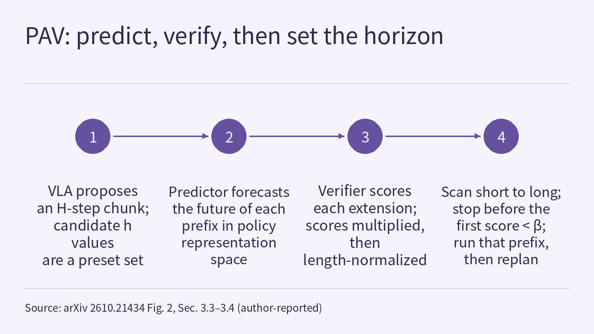
Action chunking lets a VLA generate a stretch of future actions at once, so the large model is called less often. How much of that stretch to execute before looking at the world again is a separate decision: execute too little and the query count goes up; execute too much and the robot misses changes in the scene while execution errors accumulate. A preprint with authors from Seoul National University, KAIST and Dnotitia (arXiv 2610.21434, 2026-10-15) proposes a policy-aligned predictive verifier (PAV). Before executing anything, it predicts where each candidate prefix would take the robot, in the VLA’s own task-conditioned representation space, then estimates whether the task can still be completed from there, and uses that estimate to pick the execution length. The authors report that on LIBERO with π0.5 (chunk length H = 50), average success is 7.50 percentage points higher than always executing 5 steps, with 63.3% fewer queries; on three real-robot tasks average success is 74.4%, against 41.1% for the best fixed execution length. Below: how it learns per-segment judgments from episodes labelled only “success” or “failure”, what it is compared against, and where the gains shrink. All numbers are author-reported [R]; this site has not reproduced them.
The question: how much of a chunk to execute
Suppose policy π generates a chunk of length H at time t from the observation and instruction. Choosing an execution length h means executing only the first h actions, then taking a new observation after h steps and querying the policy again. The paper frames this as a trade-off between inference cost and temporal consistency on one side and responsiveness on the other. A fixed execution horizon uses the same h for every chunk and state; adaptive execution decides each time.
The paper sorts existing adaptive methods into two kinds of signal:
- Generation stability: judging from information inside the policy. AutoHorizon estimates an execution limit from action self-attention; A3 selects a horizon from action consensus and re-decoding stability, i.e. it regenerates an action with the other actions in the chunk fixed as context and checks whether it stays the same; DVAC also falls in this group and, going by its title, uses denoising variance to decide when to replan.
- Prediction agreement: comparing action-conditioned predictions with actual observations during execution. VLA-Corrector truncates and replans when predicted and observed visual dynamics persistently diverge; CheckVLA relates prediction–observation discrepancies to failure risk.
The paper’s argument is that neither kind of signal, on its own, establishes whether the task can still be completed after executing a given prefix. In the Figure 1 example, generation stability and prediction agreement stay high through a missed grasp and task failure, while the authors’ “proposal validity” triggers replanning earlier and the example ends in success. This is a single example chosen by the authors: it shows that the signals can fail, not how often that happens.
The method: predict the consequence, then verify that the task can continue
The decision target. Proposal validity V_t(h) is defined as the probability that policy π can still complete the task successfully after executing the first h actions of a fixed proposal, with “still completable” required after every extension. The set defined this way is prefix-closed: a completable trajectory has completable shorter prefixes. So V_t(h) can be written as V_t(h−1) times the conditional probability that the h-th extension is still completable. The paper splits that conditional probability into two steps: predict the future representation after execution, then verify whether that representation supports successful continuation.
The predictor. The representation z_t is extracted from the observation and instruction by the policy’s own encoder. The predictor f_θ takes z_t and the first h actions and outputs the predicted representation h steps later; its training target is the encoding of the observation after actual execution. There are two loss terms: cosine distance to the true future representation, and action-swap ranking, which requires the prediction for a different action prefix from the same task to be farther from the target than the executed prefix’s prediction by a margin m. The swapped actions are not labelled as failures.
The verifier. The verifier q_φ reads only the predicted future representation and outputs a local validity q between 0 and 1. Multiplying the q values of successive segments gives the prefix score that approximates V_t(h).
Learning per-segment judgments from episode outcomes. Training episodes carry only a final success or failure, with no per-segment labels, and a failed episode may still contain valid prefixes. The paper treats per-segment validity as latent: in successful episodes every factor is pushed up, averaged over the number of segments so that long episodes are not overweighted; in failed episodes only the overall product is pushed down, without labelling every segment a failure. The model could still fit a failed episode by lowering every segment slightly, including the valid ones. The paper therefore adds a localization prior that penalizes Σ(1 − q_i) on failed episodes. At a fixed product, minimizing this sum concentrates the reduction in a few segments.
A hypothetical example constructed by this site: a failed episode has 10 segments and the product must come down to 0.5. Option one spreads the reduction evenly, q = 0.5^(1/10) ≈ 0.933 per segment, so Σ(1 − q) ≈ 0.67. Option two lowers a single segment to q = 0.5 and leaves the rest at q = 1, so Σ(1 − q) = 0.5. Both give the same trajectory-level failure loss; the localization term favours option two, which keeps high scores on the other 9 segments. This is arithmetic to illustrate the mechanism, not data from the paper.
Choosing the execution length. At deployment the accumulated score is length-normalized by the square root of the number of blocks, so that it does not favour short prefixes merely because fewer factors have been multiplied. Candidates are then checked from shortest to longest; the scan stops at the first score below the threshold β, the longest prefix before that point is executed, and the policy is queried again from the new observation. The normalized score need not be monotone, and this rule prevents accepting anything beyond an earlier violation. A hypothetical example: with β = 0.9 and scores of 0.97, 0.94, 0.91, 0.88 and 0.92 for h = 5, 10, 15, 20 and 25, the result is h = 15; h = 25 is above 0.9 but is not accepted.
Implementation (the π0.5, LIBERO, H = 50 configuration). The final prefix hidden states before action denoising are taken from the policy’s PaliGemma language model; masked mean pooling, masked max pooling and the last non-padding token each give a 2,048-dimensional vector, which are concatenated with the 32-dimensional state into 6,176 dimensions and projected to 128. The VLA parameters remain unchanged. The 50 × 7 action sequence is split into 10 blocks of 5 steps and fed through a GRU recurrence, so one rollout evaluates all 10 candidate lengths. The verifier reads neither an action embedding nor the GRU hidden state; action information reaches the score only through the predicted consequence. The module has 2,011,208 parameters, including a completion head used only in training. The training data are 150 episodes for each of the 40 tasks across the four LIBERO suites, 6,000 in total, with the execution length sampled uniformly from {5, 10, …, 50} at every query; splitting by initial state gives 4,200 / 840 / 960 training, validation and test episodes. The threshold is β = 0.9, the localization weight 0.01 and the swap-ranking margin 0.1. The authors state that, “to our knowledge”, this is the first method to combine prefix-conditioned future prediction with proposal-validity estimation for adaptive action-chunk execution.
Results: against what, and at how many queries
Each action-chunk generation counts as one query; the query figures in the tables are means per episode. LIBERO uses 50 trials per simulation task. The table below excerpts the paper’s Table 1 (average success across the Spatial, Object, Goal and Long suites); entries marked † are published reference results whose protocols may differ.
| Setting | Method | Average success (%) | Queries / episode |
|---|---|---|---|
| π0, H = 50 | Fixed h = 5 | 92.10 | 34.6 |
| π0, H = 50 | Fixed h = 10 | 93.05 | 17.2 |
| π0, H = 50 | Fixed h = 50 | 76.05 | 4.4 |
| π0, H = 50 | AutoHorizon | 94.05 | 10.6 |
| π0, H = 50 | PAV | 94.30 | 12.3 |
| π0.5, H = 10 | Fixed h = 10 | 97.50 | 16.1 |
| π0.5, H = 10 | AutoHorizon | 97.8 | 27.8 |
| π0.5, H = 10 | A3 | 97.55 | 16.4 |
| π0.5, H = 10 | DVAC † | 98.00 | 18.6 |
| π0.5, H = 10 | VLA-Corrector † | 97.80 | Not reported |
| π0.5, H = 10 | PAV | 98.10 | 16.8 |
| π0.5, H = 50 | Fixed h = 5 | 87.15 | 38.1 |
| π0.5, H = 50 | Fixed h = 10 | 87.45 | 19.2 |
| π0.5, H = 50 | Fixed h = 50 | 56.80 | 5.4 |
| π0.5, H = 50 | AutoHorizon | 94.45 | 12.7 |
| π0.5, H = 50 | PAV | 94.65 | 14.0 |
PAV has the highest average success in all three settings. Against fixed horizons the gap is largest with π0.5 at H = 50: 7.50 points above h = 5 (94.65% vs 87.15%), with queries falling from 38.1 to 14.0, 63.3% fewer; executing all 50 steps at once reaches only 56.80%. At H = 10 there are only two candidates, 5 and 10; PAV goes from 97.50% to 98.10% at 16.8 vs 16.1 queries.
Against the strongest adaptive baseline, AutoHorizon, the gap is much smaller: 0.25 points higher with π0 at H = 50 but with more queries (12.3 vs 10.6), and 0.20 points higher with π0.5 at H = 50 at 14.0 vs 12.7 queries. The table gives no confidence intervals, and this site does not read gaps this small as a ranking. The appendix adds a comparison at a similar query count: at β = 0.91, PAV reaches 89.45% with 19.7 queries, against 87.45% with 19.2 for fixed h = 10, a 2.00-point gain. π0.5 at H = 50 uses a separate checkpoint fine-tuned with H = 50, and the authors state that checkpoint differences prevent isolating the effect of chunk length.
On RoboTwin 2.0 the paper uses π0.5 with its default H = 32, fixed horizons h ∈ {4, 8, 20, 32} and 50 evaluation episodes per task (Table 2):
| Method | Selected 16 success (%) | Selected 16 queries | All 50 success (%) | All 50 queries |
|---|---|---|---|---|
| Fixed h = 4 | 17.38 | 181.3 | 27.40 | 136.5 |
| Fixed h = 8 | 46.75 | 75.0 | 55.76 | 54.5 |
| Fixed h = 20 | 47.88 | 28.2 | 55.16 | 20.8 |
| Fixed h = 32 | 35.38 | 19.7 | 43.64 | 14.6 |
| DVAC † | 41.6 | Not reported | Not reported | Not reported |
| PAV | 54.13 | 59.8 | 58.64 | 58.5 |
On the 16-task subset used by DVAC, PAV reaches 54.13%, against 47.88% for the best fixed horizon (h = 20) and a quoted 41.6% for DVAC; across all 50 tasks, PAV reaches 58.64% against 55.76% for the best fixed horizon (h = 8). Query counts belong in the same reading: on the 16-task subset PAV uses 59.8 queries per episode, about 2.1 times h = 20’s 28.2 (this site’s calculation); across all 50 tasks it is close to h = 8 (58.5 vs 54.5). The appendix states that the RoboTwin verifier uses β = 0.91 and includes a task embedding, unlike the LIBERO configuration; that the h = 32 baseline comes from a separate evaluation, so its episode-level initial conditions are not guaranteed to be paired with the other methods; and that DVAC is an external reference under its published H = 50 policy and evaluation protocol. AutoHorizon and A3 do not appear in the RoboTwin table.
The real-robot experiments use a 7-DoF Franka Panda with front, wrist and right-side RGB cameras. For each task, π0.5 is fine-tuned from its base checkpoint on teleoperated demonstrations (H = 50), and robot rollouts are then collected to train the verifier. The three tasks are placing an orange cube in a tray (Place Cube in Tray), stacking it on a green cube (Stack Cubes) and pressing a red emergency button (Press Button); object positions are randomized within a 50 cm × 50 cm workspace, with 30 trials per task (Table 6):
| Method | Place Cube in Tray (%) | Stack Cubes (%) | Press Button (%) | Average success (%) | Average replans | Average horizon |
|---|---|---|---|---|---|---|
| Fixed h = 5 | 16.7 | 10.0 | 23.3 | 16.7 | 69.58 | 5.00 |
| Fixed h = 10 | 66.7 | 16.7 | 40.0 | 41.1 | 36.54 | 10.00 |
| Fixed h = 30 | 23.3 | 43.3 | 53.3 | 40.0 | 11.97 | 30.00 |
| Fixed h = 50 | 26.7 | 33.3 | 50.0 | 36.7 | 6.91 | 50.00 |
| PAV | 80.0 | 66.7 | 76.7 | 74.4 | 12.87 | 30.22 |
PAV is highest on all three tasks, averaging 74.4%; the best fixed horizon, h = 10, reaches 41.1% with 36.54 replans on average, against 12.87 for PAV. Compared with h = 30, which replans a similar number of times (11.97), average success rises from 40.0% to 74.4%, while PAV’s average execution length is 30.22 steps. The authors take this as evidence that the benefit comes from varying the execution length rather than switching to another constant one. Points to note: the real-robot table contains only fixed-horizon baselines and no adaptive method; there are 30 trials per task and no confidence intervals; and the main text read here does not give the number of rollouts used to train the real-robot verifier (those details are in Appendix E, which is not in the text this site read). Fixed h = 5 averages only 16.7%, far below h = 10, and the text read does not explain why.
Ablations: which parts matter, and how sensitive the threshold is
The following analyses all use LIBERO with π0.5 at H = 50, the same policy checkpoint and the same rollout data (Tables 3 and 12):
| Variant | Average success (%) | Queries / episode |
|---|---|---|
| Direct: no future prediction, scoring from current representations and actions | 84.55 | 22.3 |
| Prediction in DINOv2 feature space | 87.00 | 22.2 |
| Without future alignment | 85.30 | 23.99 |
| Without action-swap ranking | 85.70 | 24.26 |
| Without the localization prior | 83.65 | 25.60 |
| Full PAV | 94.65 | 14.0 |
The full method is 7.65 to 11.00 points above every variant, with fewer queries. The DINOv2 comparison keeps the same prediction–verification pipeline and changes only the representation space; the authors read it as support for retaining task-conditioned information when evaluating proposals. Does the predictor actually look at the actions? On held-out episodes, with the current input and observed target held fixed, the cosine similarity between prediction and true future is 0.9401 with the executed actions, 0.5304 with another action sequence from the same task, 0.4816 with reversed actions and 0.4103 with zero actions; broken down by prediction horizon, the executed actions give the closer prediction in 89.3%–95.2% of pairs.
The threshold, by contrast, is quite sensitive. Table 11 keeps the trained verifier fixed and varies only β. Its caption states that queries in the sweep are counted as total selections divided by 2,000 episodes, and that “the default row uses the PAV results from the main paper”, so the 94.65% at β = 0.90 was not produced in the same sweep run as the other four rows:
| β | Average success (%) | Queries / episode | Mean horizon |
|---|---|---|---|
| 0.88 | 82.75 | 13.8 | 15.200 |
| 0.89 | 85.65 | 15.1 | 13.443 |
| 0.90 (default) | 94.65 | 14.0 | 12.783 |
| 0.91 | 89.45 | 19.7 | 9.685 |
| 0.92 | 88.30 | 25.1 | 7.614 |
Compared with the default row, the rows that move β by just 0.01 are 5.20 to 9.00 points lower in average success, which makes the default look like a narrow peak. Both the drop and the apparent peak, however, compare sweep rows with a default row taken from a different run, not rows within a single sweep. The text read does not say how β = 0.90 was chosen, or whether data independent of the evaluation episodes were used to choose it. When the method is moved to a new task or policy, this threshold deserves its own check.
On overhead: across four policy and chunk configurations, verifier GPU computation takes 0.90–2.49 ms, or 0.45%–1.24% of action-generation time (180.34–216.95 ms). The authors state that this is GPU computation time, not end-to-end control-loop latency.
How this relates to existing articles on this site
Physical AI Lab 0.3: See, Think, Act describes how, in the π0 paper, a robot running at 50 Hz re-runs inference after every 25 actions, roughly every 0.5 seconds: a fixed execution horizon. PAV lets that interval vary with each proposal, and 0.3’s rule still applies: an interval belongs only to the system and configuration that reports it.
Physical AI Lab 1.6: Imitation Learning covered action chunking and how errors snowball. The PAV paper likewise notes that executing a whole chunk without new observations lets execution errors accumulate; in Table 1, executing all 50 steps at once gives the lowest success (76.05% and 56.80%), an example of this point on LIBERO.
VeriVLA, covered earlier on this site, uses the change between two action samples to trigger verification, then a latent world model picks one of 10 candidate chunks by predicted progress; RESETTLE steps in only when two samples keep disagreeing. Those answer “which chunk” and “when to intervene”; PAV answers “how much of this chunk to execute”. The generation-stability signals the PAV paper discusses include A3’s action consensus and re-decoding stability, which is close in spirit to the sample differences those two papers use. The PAV paper does not evaluate either method, however, and the three use different benchmarks and settings, so their numbers cannot be compared directly.
When reading the RoboTwin table, the unpaired h = 32 baseline and DVAC’s different protocol can be checked item by item with the questions from Physical AI Lab 1.8: Evaluation: conditions, trial counts, and whether runs are paired.
Limitations
- This is an arXiv preprint; all numbers are author-reported [R], and this site has not reproduced them. The authors state that the implementation will be submitted as supplementary material; the text read gives no public code address.
- The simulation results come from LIBERO and RoboTwin 2.0. The real-robot evidence covers one platform (Franka Panda), three tasks and 30 trials each, with fixed-horizon baselines only. Neither the simulation results nor these real-robot results are a hardware safety validation.
- Against AutoHorizon, PAV is only 0.20–0.25 points higher in the two LIBERO H = 50 settings, with more queries; the table gives no confidence intervals.
- Baselines marked † are published reference results whose protocols may differ; RoboTwin’s h = 32 baseline is not paired with the other methods, and DVAC uses an H = 50 policy.
- The verifier is trained separately for each policy configuration and benchmark (in simulation, tasks within one configuration and benchmark share one verifier) and needs rollouts collected with random execution lengths; the LIBERO configuration used 6,000 episodes. The LIBERO and RoboTwin configurations differ (β, task embedding).
- The threshold β is sensitive around its default, and the text read does not describe how it was chosen. Table 11’s default row reuses the main-paper results rather than coming from the same sweep run as the other rows, so the 5.20–9.00-point drop is a cross-run comparison. The 0.90–2.49 ms overhead is GPU computation only.
- The HTML text read is cut off at Table 13 in Appendix C.4, and Appendix E (real-robot hardware and training details) is not included. Several table numbers in the main text do not match the table captions; for example, the RoboTwin results are cited as Table 3 (they are in Table 2) and the cosine similarities as Table 5 (they are in Table 4). This article cites the tables by their captions.
Links
- Policy-Aligned Predictive Verification for Adaptive VLA Action-Chunk Execution (arXiv 2610.21434)
- Full paper (HTML)
- Physical AI Lab 0.3: See, Think, Act — Putting Each Rate Back in Its Own System
- Physical AI Lab 1.6: Imitation Learning — Working Out How an Error Rolls Out of the Demonstrations’ Coverage, Then Putting the ACT, Diffusion Policy and Data Scaling Numbers Back in Their Own Conditions
- Physical AI Lab 1.8: Evaluation — Splitting a “Net Gain of 2” into a Paired Table, Then Checking the Failure Labels and Random Seeds
- Frontier Radar | VeriVLA: two samples decide when extra computation is worth it, then a latent world model picks one of 10 candidate action chunks by predicted progress
- Frontier Radar | RESETTLE: step in only when a frozen policy’s two action samples keep disagreeing, then execute one demonstration-guided correction
- Physical AI Lab: a physical AI course where every number can be checked (course outline)