Flow-matching VLAs sample action chunks from Gaussian noise: with the same observation and instruction, a different noise seed can yield an action chunk of different quality, yet at deployment the policy usually executes a single sample. VeriVLA, a preprint from a University of Hong Kong team (arXiv 2610.21985, 2026-10-15), treats this randomness as a resource to select from. Two initial samples give a training-free “two-axis” trigger score that decides whether the current state is critical enough to justify extra computation. Once triggered, the policy samples 8 more chunks for 10 candidates in total, and a JEPA-based latent world model predicts each candidate’s future latent state and change in task progress; the candidate with the largest predicted progress is executed. The authors report that the average completion score over three real-robot tasks rises from 50.8% to 65.5%, with each triggered decision costing an extra 326 ms on a single RTX 4090. RoboTwin 2.0 and LIBERO also improve in simulation, but the main RoboTwin 2.0 table uses always-on verification, not the trigger. All numbers below are author-reported [R]; this site has not reproduced them.
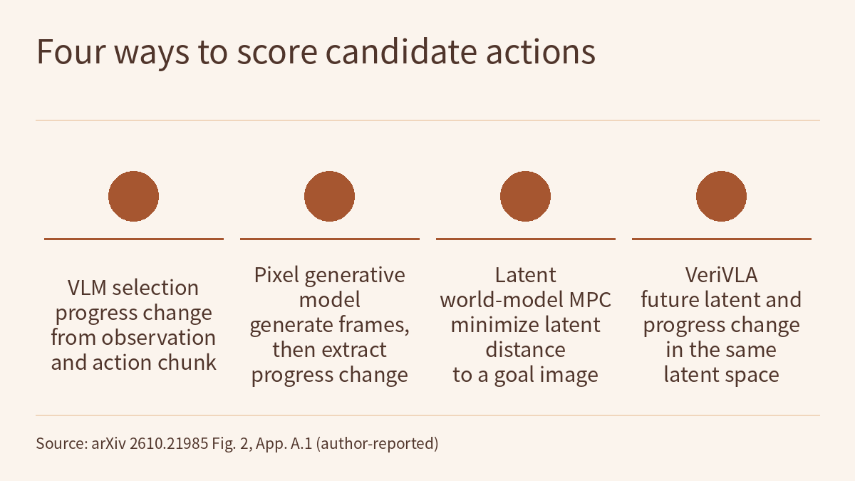
The paper’s Figure 2, appendix Table 6 and related work (§2, §3.4) sort similar methods into several kinds. RoboMonkey fine-tunes a 7B VLM on synthetic action preferences and scores directly from the current observation and the action chunk. GPC-RANK and DreamAvoid first generate future pixels and then extract a reward or progress from them, in two stages. Latent world models such as DINO-WM and V-JEPA 2-AC plan by search and need a goal image. VeriVLA keeps the world model but produces the future latent state and the progress change in one step in the same latent space, with no pixel reconstruction and no goal image. The authors’ reasoning: how far an action chunk advances the task is a scalar judgment, and most camera pixels are irrelevant to it; pixel-level world models are slow to generate, and they must solve the harder problem of image generation before the easier problem of progress estimation, which ties verification quality to generation quality.
When extra computation is worth it: two samples, two axes
The authors observe that policy variance is not uniform along a task: repeated sampling in LIBERO shows higher action variance as the end-effector approaches contact-rich regions, and failures tend to occur in these high-variance segments (Figure 1 of the paper). The trigger is therefore designed to meet two conditions: activate in contact-rich regions, where manipulation is more complex (C1), and activate in states where repeated sampling yields diverse candidates, giving the verifier real alternatives (C2).
At each decision step the policy first draws k = 2 action chunks. To avoid a bias toward fast-moving stages, each chunk is normalized by its own average action magnitude. Two quantities are then computed:
- Temporal axis (C1): the mean squared change between consecutive actions within each chunk, averaged over the k samples, written T_temp.
- Sample axis (C2): the mean squared deviation of each sample from the k-sample mean at each step, written T_cross; the authors say it is motivated by AdaFlow’s variance-adaptive computation.
Before deployment in a new environment, the base policy is rolled out for a small number of episodes and T_temp and T_cross are computed at every timestep, giving two empirical reference distributions. At run time both values are converted to percentiles within their distributions, the larger one is taken, τ = max(τ_temp, τ_cross), and verification triggers when it exceeds the threshold τ0, so either axis alone can trigger it. τ0 is the trigger’s only hyperparameter. When the trigger is inactive, no further samples are drawn and the first sample is executed directly.
In simulation the authors assess the trigger with two diagnostics. Status AUC measures agreement between the trigger score and a “critical moment” label built only from privileged simulator state: Gaussian kernels are placed where gripper–object or object–object contact flips, summed and clipped to 1, then binarized at 0.5, without using the images or actions the triggers see. Variance Correlation is Spearman’s ρ between the trigger score and a reference variance estimated from K samples per state. According to the appendix, the DINO baseline is evaluated together with the other methods on the LIBERO-Plus perturbation set.
| Trigger | Status AUC | Variance Correlation | Samples k / added latency (ms) |
|---|---|---|---|
| Random | 0.487 | – | – |
| DINOv2 features + MLP (trained) | 0.702 | 0.630 | 0 / 0 |
| Action chunk entropy (ACE) | 0.588 | 0.716 | 2 / 14 |
| T_temp only | 0.704 | 0.789 | 1 / 0 |
| T_cross only | 0.694 | 0.877 | 2 / 14 |
| Two-axis trigger | 0.727 | 0.887 | 2 / 14 |
The temporal component has the higher Status AUC and the sample component the higher variance correlation, which the authors read as complementary signals; combined, both scores are slightly above either component. These diagnostics measure how well the trigger score tracks contact moments and policy variance, not closed-loop success; the closed-loop trade-off between success and computation is evaluated separately in Figure 6. On the real robot the authors set the threshold so that verification turns on during contact-rich phases. The exact threshold and per-task trigger rates appear only in Figure 5b; the text this site read gives no values.
How candidates are scored: predicting in latent space how far a chunk advances the task
The paper defines the quality of an action chunk as the change in task progress between before and after executing it, the delta progress Δp = p_{t+H} − p_t. The authors argue that, unlike absolute progress, the change corresponds directly to the effect of that chunk.
The verifier is built on the JEPA world-model framework. The visual encoder is a frozen pretrained V-JEPA 2 that compresses the current observation into a latent representation; an action-conditioned autoregressive predictor, pretrained on 23k trajectories from the DROID dataset, predicts how the latent state evolves under the robot’s actions. To adapt it to a specific robot, the authors add embodiment-specific state and action encoders and split each action chunk of horizon H evenly into M sub-chunks for a multi-step rollout (M = 5 in the hyperparameter table for the real-robot experiments).
A progress-prediction branch sits on top. The same state transition is positive progress for “closing the closet” and negative progress for “opening the closet”, so progress prediction needs task information: each task gets a learnable query token, and for every sub-chunk the predictor first predicts the next latent state, then the corresponding progress change. An attention mask keeps latent-state prediction from seeing this task token, so that task semantics do not leak into the dynamics model and the latent dynamics stay task-agnostic.
Progress estimation is the primary training objective. On each sub-chunk a Huber regression loss fits the progress targets and a pairwise ranking loss over same-task pairs preserves their ordering (the ranking loss follows DreamAvoid), plus an L1 latent-prediction loss defined as in V-JEPA 2-AC; training uses both teacher forcing and self-forcing. Absolute progress is labeled automatically with Robometer, and the change is computed from those labels. For data, each real-robot task uses 50 demonstrations to fine-tune the base policy π0.5, plus another 50 policy rollouts labeled with Robometer; all tasks in an environment share one verifier, trained on a single H800. The simulation experiments use the same protocol.
At inference the predictor conditions only on its own previously predicted latent frames and rolls out autoregressively over each candidate’s M sub-chunks, producing M progress changes; these are summed, and the candidate with the largest cumulative predicted progress is executed. To make this practical on a real robot, three latency optimizations are applied cumulatively: reusing the KV cache throughout the autoregressive rollout; overlapping independent computations, such as generating candidate chunks in parallel and encoding latent features while the VLA generates actions; and PyTorch-level optimizations including pre-compilation. Figure 5a shows the KV cache giving the largest reduction; the text gives no per-stage numbers.
Results: three real-robot tasks and two simulation benchmarks
The real-robot experiments use an AgileX PiperX dual-arm robot with one front RealSense D455 and two wrist RealSense D435 cameras. The three tasks are pen insertion (pick up a pen and insert it into a yogurt bottle), pipetting (transfer liquid from the right bottle to the left with a pipette) and apple placement (pick up an apple and place it in a container); one is single-arm and two are dual-arm. Each method is run 50 times per task, with k = 2 for the trigger and K = 10 for the verifier. The completion score is awarded by stage: pen insertion and apple placement each have two stages worth 0.5 points, and if the apple needs several attempts to be placed, that stage earns only 0.25; pipetting has four stages worth 0.25 each.
| Method | Rank loss ↓ | Huber loss ↓ | Pen insertion (%) | Pipetting (%) | Apple placement (%) | Average (%) |
|---|---|---|---|---|---|---|
| π0.5 (single sample) | – | – | 45.0 | 52.5 | 55.0 | 50.8 |
| + RoboMonkey (VLM verifier) | 1.19 | 0.37 | 49.0 | 55.5 | 63.5 | 56.0 |
| + GPC-RANK (pixel-level world-model verifier) | 1.18 | 0.30 | 46.0 | 54.5 | 58.0 | 52.8 |
| + VeriVLA | 1.09 | 0.25 | 60.0 | 63.5 | 73.0 | 65.5 |
The two losses are offline validation metrics: rank loss measures the ability to order samples within a task, Huber loss the regression accuracy of the progress change; the completion score is the closed-loop result. The RoboMonkey baseline’s training objective was adapted to delta-progress estimation. The authors explain the gaps this way: RoboMonkey is competitive on tasks that need only coarse localization, such as apple placement, but struggles with fine-grained manipulation, “likely” because its VLM lacks an explicit understanding of world dynamics; GPC-RANK does well when estimating progress from real observations but degrades on frames generated at test time, indicating that generation quality becomes the bottleneck. The text this site read does not say whether the baselines use the same trigger and the same number of candidates, and gives no confidence intervals.
The ablation (Table 4) uses the same three real-robot tasks, with the visual encoder pretrained in every variant. Removing the latent-state prediction objective and predicting only the progress change lowers the average completion score from 65.5% to 55.2% (pen 52.0, pipetting 55.5, apple 58.0), slightly below the RoboMonkey baseline’s 56.0%. Initializing the predictor randomly instead of pretraining it on DROID lowers the average to 59.5% (54.0, 61.0, 63.5). The authors note that apple placement, which demands more generalization, drops most, while pipetting, where the bottle positions are almost fixed, drops less.
In simulation each method is again run 50 times per task. RoboTwin 2.0 uses Hy-Embodied-0.5-VLA as the base policy on five fine-grained tasks with relatively low baseline success rates; both result sets in Table 2 use always-on verification, and in the Clean2Random setting the policy and verifier are trained only on clean data and evaluated in randomized environments. LIBERO uses two base policies, π0.5 and StarVLA-GR00T, over 40 tasks; each base policy has its own verifier weights, shared across the 40 tasks. The text this site read does not state whether the LIBERO results use the trigger or always-on verification.
| Benchmark (base policy) | Baseline (%) | + RoboMonkey (%) | + GPC-RANK (%) | + VeriVLA (%) |
|---|---|---|---|---|
| RoboTwin 2.0 Clean, five-task average (Hy-VLA) | 66.4 | 65.2 | 68.8 | 73.6 |
| RoboTwin 2.0 Clean2Random, five-task average (Hy-VLA) | 62.8 | 64.8 | 64.8 | 69.6 |
| LIBERO, average of four suites (π0.5) | 96.9 | 97.3 | 95.3 | 97.6 |
| LIBERO-10 (π0.5) | 92.4 | 94.0 | 89.0 | 94.0 |
| LIBERO, average of four suites (StarVLA-GR00T) | 96.2 | 96.3 | 96.7 | 97.2 |
| LIBERO-10 (StarVLA-GR00T) | 91.0 | 91.6 | 92.4 | 93.6 |
With 50 trials per RoboTwin 2.0 task, one trial corresponds to 2 percentage points; over 250 trials for the five tasks, the 7.2-point gain in Clean amounts to about 18 additional successes and the 6.8-point gain in Clean2Random to about 17 (this site’s arithmetic). Task by task, VeriVLA does not lead everywhere: on Seal in Clean2Random it scores 78% against GPC-RANK’s 80%, and in Clean RoboMonkey’s average falls below the base policy’s. On LIBERO the gain is concentrated in LIBERO-10, the suite that is not yet saturated, where VeriVLA and RoboMonkey both reach 94.0% with π0.5. The trigger’s effect in simulation is shown in Figure 6: in the Clean setting a single threshold is adjusted for all tasks so that roughly a fraction r of decision steps trigger verification. The authors state that always-on verification raises success on all five tasks and that the trigger retains much of the gain on the first four tasks while reducing computation; the figure’s values do not appear in the text this site read.
Latency and memory: what the 326 ms includes
Appendix Table 9 breaks down the real-robot deployment, with the policy and the verifier on the same RTX 4090:
| Component | Latency (ms) |
|---|---|
| VLA policy | 82 |
| Two-axis trigger (k = 2) | 14 |
| Additional sampling (K − k = 8 more candidates) | 80 |
| Verifier forward (all K = 10 candidates) | 246 |
| Total per decision, not triggered | 96 |
| Total per decision, triggered | 422 |
| Additional latency, verification only | 326 |
The 326 ms is the sum of additional sampling and the verifier forward pass (80 + 246) and excludes the 14 ms trigger; an untriggered decision takes 82 + 14 = 96 ms and a triggered one 422 ms (this site’s arithmetic). On memory, the VLA policy uses 9.8 GB and the verifier forward pass over 10 candidates 8.7 GB, 18.5 GB combined. The average added latency per action chunk depends on the trigger rate and is shown only in Figure 5b. The text this site read does not say whether the robot waits during a triggered decision’s computation or how that computation overlaps with chunk execution.
How this relates to other pages on this site
Physical AI Lab 1.6: Imitation Learning explained that diffusion policies can learn a multi-modal action distribution, with several correct ways to handle the same scene, instead of averaging a left and a right detour into a collision. VeriVLA looks at the other side of that randomness at deployment: only one sample is executed each time, and the sample drawn may be a poor one, so at critical moments it draws several and picks one. The compounding error discussed in 1.6 is also one of this paper’s starting points: a poor action chunk can lead directly to failure or let the trajectory drift out of distribution.
Two recent Radar articles each overlap with part of it. Frontier Radar | RESETTLE also decides when to intervene from two samples of a frozen policy, but it steps in only when the two samples keep disagreeing; once triggered, it retrieves a same-task demonstration and executes a single corrective action. VeriVLA uses two axes, within-chunk temporal variation and cross-sample variance, triggers when either exceeds its threshold, and then picks one of 10 candidates. Frontier Radar | LiteNWM likewise scores candidates in latent space without rendering RGB frames for each one, but its candidates are navigation trajectories, whereas VeriVLA predicts progress on manipulation tasks. The three papers use different benchmarks, base policies and hardware and are not compared directly, so their numbers cannot be ranked against each other.
When reading VeriVLA’s numbers, the questions from Physical AI Lab 1.8: Evaluation apply: the real-robot average is the mean of three tasks’ completion scores, which include partial credit; with 50 trials per task, the text gives no per-trial gains and losses and no confidence intervals; and the main simulation table uses always-on verification, with the computational savings of the “adaptive” mode shown only in figures.
Limitations
- This is an arXiv preprint; all numbers are author-reported [R], and all authors are at the University of Hong Kong. This site has not reproduced any result.
- Reference [11] (DreamAvoid) is signed X. Fan, Y. Lu, … H. Zhao, the same initials as three authors of this paper; the paper does not state that they are the same people. The pair construction for this paper’s ranking loss follows DreamAvoid, and the DINOv2 + MLP baseline in the trigger comparison stands for DreamAvoid-style vision-based triggers (Appendix C.3). DreamAvoid itself does not appear in the closed-loop comparisons of Tables 1–3.
- Progress labels are generated automatically by Robometer, so the verifier learns the progress assigned by that reward model; the text this site read does not report how well these labels agree with human judgment.
- The main RoboTwin 2.0 results use always-on verification; the success–computation trade-off under the trigger (Figure 6) and the real-robot trigger rates (Figure 5b) are given only as figures. The trigger diagnostics (Table 5) rely on privileged contact state from the simulator, labels that are not directly available on a real robot.
- The real-robot evaluation covers only three tasks with 50 trials each; the completion score includes partial credit, and no confidence intervals are given. The 326 ms was measured only with one RTX 4090, π0.5 and K = 10.
- Limitations stated by the authors: the verifier can only choose among the policy’s proposals, and the diversity obtained from different random seeds is still limited; the visual encoder is frozen, so its representations are not optimized for progress estimation and may miss subtle changes in object configuration, contact conditions or task completion.
- The verifier selects for predicted progress, not for collision or force constraints. Neither the simulation results nor the real-robot trials are hardware safety validation.
Links
- VeriVLA: Adaptive Test-Time Verification for Flow-Based VLAs with Latent World Models (arXiv 2610.21985)
- Full paper (HTML)
- Physical AI Lab 1.6: Imitation Learning — Working Out How an Error Rolls Out of the Demonstrations’ Coverage, Then Putting the ACT, Diffusion Policy and Data Scaling Numbers Back in Their Own Conditions
- Physical AI Lab 1.8: Evaluation — Splitting a “Net Gain of 2” into a Paired Table, Then Checking the Failure Labels and Random Seeds
- Frontier Radar | RESETTLE: step in only when a frozen policy’s two action samples keep disagreeing, then execute one demonstration-guided correction
- Frontier Radar | LiteNWM: encode once and jointly predict the consequences of 16 candidates and the incumbent trajectory in latent space, instead of rendering an RGB future for each
- Physical AI Lab: a physical AI course where every number can be checked (course outline)