
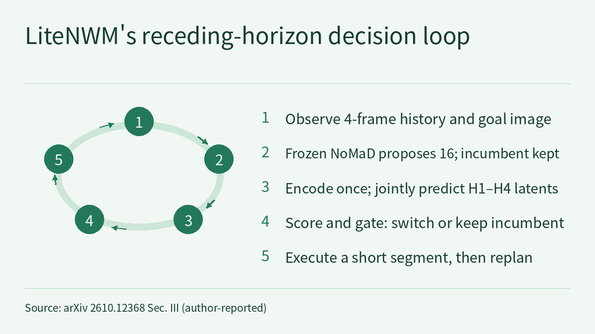
A navigation world model can predict future images for each candidate trajectory before the robot moves, then pick a trajectory based on the predicted outcome. With many candidates, however, generating an RGB future for each one becomes the dominant cost. LiteNWM (arXiv 2610.12368, 2026-10-08), a preprint by authors from Nanjing University, Imperial College London, Sony AI and Beijing University of Posts and Telecommunications, keeps the split between a navigation policy that proposes candidates and a world model that evaluates them, but moves the evaluation into latent space: the images are encoded once per decision state, the features of the 16 candidates and the incumbent τ0 over the next four steps are predicted jointly in one pass, and a learned scorer decides, relative to the current trajectory, whether to switch. The authors report a 17.56% lower macro-averaged offline trajectory error than NoMaD+NWM-XL and a 128.00× end-to-end speedup on an RTX 5090; on a real Unitree Go2 EDU, navigation success rose from NoMaD’s 43.3% to 83.3%. All numbers below are author-reported [R]; this site has not reproduced them. One point up front: the 128× is a workstation-GPU timing. On the robot’s own Jetson Orin, LiteNWM averages 2.228 s per planning call, slower than running NoMaD alone.
The bottleneck: an RGB future for every candidate
Generalist navigation policies such as GNM, ViNT and NoMaD learn goal-conditioned navigation from large, diverse robot datasets. NoMaD uses a diffusion decoder and can sample several plausible trajectories per observation (why diffusion policies can keep several correct ways of acting is covered in Physical AI Lab 1.6). The problem the authors point to is that these policies choose a trajectory without explicitly evaluating its future consequences.
Navigation World Models (NWM, Bar et al., CVPR 2025) predict future RGB observations for each candidate and select by predicted outcome. The authors explicitly treat future-conditioned trajectory reranking and the modular proposer–evaluator interface as prior art. LiteNWM addresses a narrower question: can short-horizon candidates be compared directly from action-conditioned latent features, without reconstructing an RGB future for each one?
The authors profiled component latency on an RTX 5090 with RECON-100, prediction horizon H = 4 and K = 16 candidates: candidate-wise CDiT rollout accounts for 84.8% of NoMaD+NWM-S latency and 97.6% of NoMaD+NWM-XL latency. Token-World, covered earlier on this site, also rolls out in a compact feature space without generating RGB, but it is used to simulate and evaluate VLA policy success rates; LiteNWM is used to choose a trajectory at each navigation decision point.
The method: encode once, predict four steps jointly, score against the incumbent
- Proposal. A frozen NoMaD, given a four-frame observation history and a goal image, produces K = 16 four-step candidates (the paper calls them challengers), and NoMaD’s deterministic output is retained as the incumbent τ0; K does not include τ0. A deterministic conversion writes each candidate as per-step [Δx, Δy, Δψ].
- Shared encoding. A frozen DINOv3 encoder plus a lightweight adapter encodes the history and goal once per state, shared by all candidates.
- Joint prediction. An action encoder integrates cumulative poses in SE(2); pose-conditioned warping initializes the queries, six factorized blocks refine them, and future latent features for all four horizons H1–H4 come out in one pass, with no autoregressive feedback between horizons. The predictor does not take the goal as input; it is supervised by frozen DINOv3-plus-adapter features of the actual future.
- Scoring and acceptance gate. The scorer combines the predicted futures, the current state, the goal feature and the context of the whole proposal set to predict each candidate’s change relative to τ0 in ATE, RPE, FDE and a combined measure J (J = 0.4 ATE + 0.6 FDE). The predictor and the scorer are each three-member ensembles, using a conservative estimate of the mean plus z standard deviations. A candidate is eligible only if it passes physical and proposal-support checks, the conservative estimates of both ATE and J decrease, the probability of a dual improvement is high enough and the probability of harm is low enough; if no candidate qualifies, τ0 is kept. The default offline configuration adds one CEM refinement iteration (CEM1).
- Execution. Receding horizon: at each control cycle the system observes, proposes, predicts and selects, executes a short segment of the chosen trajectory, then replans. All components stay frozen during deployment, and NoMaD is not fine-tuned.
To swap in another navigation policy, MBRA, a deterministic adapter maps MBRA’s output to the same four-step action representation, without proposer-specific retraining or recalibration.
Offline: lower error, and what the ablations and the gate show
The offline evaluation uses fixed development cohorts from three datasets, RECON, SCAND and SACSoN, with 100 query states each and four proposal seeds, for 1,200 state–seed evaluations; every method starts from the same pool of 16 NoMaD candidates. Errors are normalized by each dataset’s average waypoint spacing. Three-domain macro ATE: NoMaD+NWM-XL 0.5538, LiteNWM (CEM1) 0.4566, a 17.56% reduction; per domain the reductions are 25.21% (RECON), 14.98% (SCAND) and 14.71% (SACSoN). SR@1 is higher than NoMaD+NWM-XL by 6.5, 3.5 and 7.0 percentage points; the authors state that SR@1 measures offline endpoint agreement (normalized FDE ≤ 1), not closed-loop navigation success.
The authors also flag a fairness issue themselves: NWM’s MPC/CEM and terminal-frame objective were designed for eight-step rollouts, which may limit their effectiveness at H = 4, and absolute errors are not directly comparable with the original NWM results, which use length-eight trajectories.
The ablation swaps the predictive features on a fixed pool of 16 candidates, with a separately matched scorer for each (three-domain macro, lower is better). This is a diagnostic set-up, not the same configuration as the default CEM1 result of 0.4566 above:
| Variant | ATE | RPE | FDE |
|---|---|---|---|
| No predicted future | 0.4790 | 0.2596 | 0.6743 |
| Static DINO repeat | 0.4803 | 0.2610 | 0.6763 |
| Predicted H4 only | 0.4662 | 0.2529 | 0.6500 |
| Predicted H1–H4 | 0.4431 | 0.2316 | 0.6440 |
| H1–H4, candidates and futures mismatched | 0.4925 | 0.2672 | 0.6996 |
- Predicted futures beat both controls. When the pairing between candidates and their predicted futures is shuffled, macro ATE rises by 0.0294 (95% paired cluster-bootstrap interval [0.0175, 0.0415]), which the authors take as evidence that the scorer uses the correctly paired predictions.
- The authors state that H4 captures most of the gain and the intermediate horizons add a smaller improvement. Under an alternative grouping, the appendix gives an H4-only minus H1–H4 ATE difference of +0.0031 with a 95% interval of [−0.0014, 0.0065], which spans zero, so that analysis does not confirm the extra gain from the intermediate horizons.
- The acceptance-gate diagnostic uses a historical CEM3 configuration: the gate lowers the harmful replacement rate from 23.00% to 9.92% and replacement coverage from 100% to 64.83%, but the no-gate minus gated macro ATE difference is −0.00409 with a 95% interval of [−0.00912, 0.00076], which includes zero. The gate mainly reduces harmful replacements; it is not shown to lower average error.
- In the fixed pool, a candidate with lower ATE than the incumbent exists in 98.42% of state–seed observations; LiteNWM’s selection lowers ATE in 49.75%, raises it in 8.42% and keeps the incumbent in 41.83%.
With the same frozen evaluator attached to MBRA, three-domain macro ATE falls from 0.600 to 0.503, or 16.2%; per domain the reductions are 6.9%, 23.0% and 16.8%.
Two sets of timings: 128× on an RTX 5090, 2.2 s on a Jetson Orin
The paper has two sets of latency figures with different hardware, configurations and timing boundaries, and the authors report them separately. This is the rule practised in Physical AI Lab 0.3: a timing belongs only to the system it was measured on.
| Method | RTX 5090, end-to-end per state (s) | Jetson Orin onboard, mean per planning call (s) |
|---|---|---|
| NoMaD | 0.121 | 0.651 (302 calls) |
| NoMaD+NWM-S | 11.653 | 235.038 (22 calls, DDIM-30, one rollout) |
| NoMaD+NWM-XL | 88.449 | not reported |
| LiteNWM | 0.691 | 2.228 (311 calls; median 2.085, P95 3.883) |
- The RTX 5090 column was measured with RECON-100, H = 4 and K = 16. The timing covers proposal generation, future evaluation, scoring, refinement and final selection; LiteNWM’s figure also amortizes initialization and 30 warm-up states over the 100 evaluated states. In the same table, LiteNWM uses 0.0277 Wh of GPU energy and 2,459 MiB of peak VRAM per state, against 14.0695 Wh and 13,776 MiB for NoMaD+NWM-XL; GPU energy excludes whole-robot consumption. 88.449 ÷ 0.691 is about 128, consistent with the authors’ 128.00×.
- The Jetson Orin column is internal planning latency from the robot logs, covering shared encoding, proposal, future evaluation, scoring, conditional refinement or recovery, and final selection, but not model initialization or robot motion. Onboard, CEM is skipped when the initial pool meets the acceptance conditions; otherwise up to three refinement rounds run. Of 311 calls, four used two rounds and 19 used three.
- From the table means, this site calculates that onboard LiteNWM takes about 3.4 times as long per planning call as NoMaD (2.228 ÷ 0.651); this is not a ratio given in the paper. The “onboard” in the title corresponds to Appendix F-C: LiteNWM runs on the Go2 EDU’s onboard Jetson Orin, where evaluating the candidates still costs more time than running NoMaD alone.
For how other edge-inference latency figures break down, see Frontier Radar deep dive | Edge and real-time.
Real robot: 30 trials per method on a Go2 EDU
The deployment platform is a Unitree Go2 EDU, and the navigation policies receive only monocular RGB observations and an RGB goal image. Each of three scenes has 10 trials per method, 30 per method in total. A trial succeeds if, before a collision, a corrective intervention or an abnormal termination, the robot enters a calibrated 1.0 m goal radius with a visible, goal-consistent target observation and a yaw error within 60°; that state must persist for at least 1 s or be followed by a normal stop, and merely passing the target does not count.
| Scene | NoMaD success rate | NoMaD SPL | LiteNWM success rate | LiteNWM SPL |
|---|---|---|---|---|
| Open indoor | 70.0% | 0.642 | 90.0% | 0.890 |
| Cluttered indoor | 40.0% | 0.397 | 90.0% | 0.889 |
| Outdoor courtyard | 20.0% | 0.187 | 70.0% | 0.651 |
| Overall | 43.3% | 0.409 | 83.3% | 0.810 |
SPL is averaged over all trials, with failures scored as zero. The real-robot comparison is only between LiteNWM and NoMaD. NoMaD+NWM-S was deployed on the robot only in two exploratory runs: even with DDIM reduced to 30 steps, they averaged 234.0 s and 236.5 s per planning decision (over 13 and 9 decisions), and the authors exclude them from the success-rate comparison. Ten trials per scene is a small sample, and the paper text supplied gives no confidence intervals for the real-robot results; the questions to ask of small comparisons like this are worked through in Physical AI Lab 1.8.
Limitations
- LiteNWM is a preprint; every number is author-reported [R]. This site has not reproduced any of them, and the paper text read does not mention a code or model release.
- The paper contains two numerical inconsistencies. The conclusion states “18.39× and 132.02× end-to-end speedups over NWM-S and NWM-XL”, while the abstract, introduction and Section IV-E give 16.86× over NoMaD+NWM-S and 128.00× over NoMaD+NWM-XL; this article uses the latter, which match the table timings. The introduction describes 221.97 s as NoMaD+NWM-XL’s end-to-end time per decision state, whereas Section IV-E attributes 221.974 s to a seven-state native-CEM diagnostic of standalone NWM-XL, and the table gives 88.449 s for NoMaD+NWM-XL.
- The predictor evaluates only local consequences within four steps. The authors state that longer routes rely on repeated replanning and do not establish prediction accuracy beyond this horizon; the proposer receives no training feedback from the evaluator, so its proposal distribution is unchanged; and more aggressive score optimization could expose model errors, particularly outside the proposal distribution.
- The offline results come from development cohorts of 100 states per domain; SR@1 is offline endpoint agreement, not a closed-loop success rate. The gate and ensemble diagnostics use a historical CEM3 configuration, and none of the six ensemble-member contrasts survives Holm correction.
- The real-robot test covers three scenes and 30 trials per method, compared only with NoMaD. The extended-route demonstrations in the appendix rely on a pre-mapped visual route that supplies a sequence of intermediate goal images; they are qualitative and not part of the success-rate table.
- The 128× and the energy figures belong only to the RTX 5090 benchmark set-up, and GPU energy excludes whole-robot consumption; on the Jetson Orin, LiteNWM’s mean planning latency is higher than NoMaD’s.
Links
- LiteNWM: Efficient Latent World Models for Onboard Visual Navigation in the Wild (arXiv 2610.12368)
- Full paper in HTML
- Frontier Radar | Token-World: rolling out a world model in VLM token space to simulate VLA policies without RGB reconstruction
- Frontier Radar deep dive | Edge and real-time: where the latency budget of VLAs and world action models goes
- Physical AI Lab 0.3: See, Think, Act — Putting Each Rate Back in Its Own System
- Physical AI Lab 1.6: Imitation Learning — Working Out How an Error Rolls Out of the Demonstrations’ Coverage, Then Putting the ACT, Diffusion Policy and Data Scaling Numbers Back in Their Own Conditions
- Physical AI Lab 1.8: Evaluation — Splitting a “Net Gain of 2” into a Paired Table, Then Checking the Failure Labels and Random Seeds
- Physical AI Lab: a physical AI course where every number can be checked (course outline)