Each pixel of an event camera works independently and emits an event only when its log-intensity change exceeds a threshold, so the sensor has sub-millisecond latency, high dynamic range and almost no motion blur, which suits fast flight. The hard part is closing the control loop with it: real event data is hard to collect at scale, and existing event simulators are slow. A preprint from the Robotics and Perception Group at the University of Zurich (arXiv 2610.38967, 2026-10-28) puts a CUDA event simulator inside a differentiable-simulation training loop and trains a quadrotor obstacle-avoidance policy that maps event frames directly to acceleration commands, with no intermediate depth estimate. The authors report convergence in about 3 hours on an RTX 5060 laptop GPU and zero-shot deployment on a real quadrotor. The real-world experiments use one indoor scene with one static obstacle, and the table records 11 flights in total. All figures below are author-reported [R]; this site has not reproduced them.
What the two existing approaches cost
The paper sorts related work into two groups and names a cost for each:
- Cascaded architecture (Bhattacharya et al.): a perception network first predicts depth from the event stream, and a separate velocity predictor maps that depth to control commands. Control performance depends on the accuracy of the intermediate depth estimate, and depth errors propagate to the control output.
- End-to-end, but pretrained offline first (Messikommer et al., approximate imitation learning): events are rendered offline to learn a task-specific event representation space, and the action decoder is then fine-tuned online. According to this paper, the offline stage takes on the order of 200 hours before online fine-tuning can begin.
The authors also argue that model-free reinforcement learning such as PPO is sample-inefficient when learning from high-dimensional visual input like events. Their approach changes two things together: event generation becomes fast enough to sit inside the training loop, and differentiable simulation lets gradients pass directly through the dynamics model to improve sample efficiency.
The event simulator: render only obstacle boundaries
The simulator does not aim for photorealism. It keeps the signal that obstacle avoidance needs: as the camera moves, obstacle boundaries shift across the image, change brightness and trigger events. Concretely:
- Obstacles are approximated by simple primitives (spheres, voxels, vertical and horizontal cylinders), and each obstacle gets a uniform, randomly sampled grayscale intensity. Ray intersections with these primitives have closed-form solutions, so every pixel can be ray-cast independently and in parallel on the GPU; a pixel takes the intensity of the nearest intersection, which preserves occlusion.
- Events are generated per control step: the grayscale frames rendered at two consecutive control steps are compared, and a pixel gets +1 if the difference exceeds the contrast threshold C, −1 if it is below −C, and 0 otherwise. The paper calls this a fast approximation of the per-pixel intensity change.
- The render resolution is only 64 × 48. At deployment, 640 × 480 real event frames are downsampled to the same resolution; the authors argue this acts as an implicit low-pass filter that suppresses sensor noise and task-irrelevant detail.
- To narrow the sim-to-real gap, the simulator adds lens distortion with the Kannala-Brandt fisheye model, using coefficients from calibrating the real camera. The positive and negative thresholds are resampled independently at every simulation step from clipped Gaussian distributions, and background-noise events unrelated to edges are triggered at random in a small fraction of pixels.
The efficiency comparison uses a 64 × 48 pinhole camera view of a scene with 200 randomly placed obstacles, a camera trajectory sampled at 15 Hz and N = 1 to 256 parallel environments, all measured on the same RTX 5060 laptop GPU. At N = 128, the authors’ simulator reaches 60,248 environment steps per second and ESIM (an OpenGL renderer with a CPU event-generation core) 4,249, about 14×. At that point it uses 138 MB of GPU memory, against ESIM’s 656 MB of host memory. The authors also benchmarked a multi-threaded CPU-only implementation of their own simulator, but the main text gives no figure for it.
How differentiable simulation trains the policy
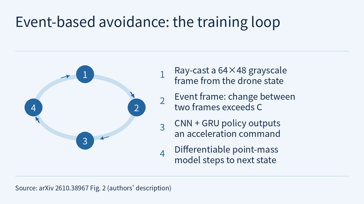
The training loop is in the paper’s Fig. 2: a grayscale frame is rendered from the quadrotor state, and two consecutive frames give the event frame; the policy (a CNN encoder plus a GRU) outputs an acceleration; a differentiable point-mass model steps the state forward; a loss is computed from state and action, and gradients flow back through the whole loop (backpropagation through time, with temporal gradient decay α = 0.4). The dynamics are not a full quadrotor model; following Zhang et al. (DiffAgile), they use a point-mass approximation.
The loss is a weighted sum of five terms:
- velocity tracking: the difference between a 2-second moving-average velocity and the target velocity, with Smooth L1, weight 1.0;
- velocity estimation: mean squared error between the network’s own velocity estimate and simulator ground truth, weight 100, used for the odometry-free setting;
- obstacle avoidance: a quadratic clearance barrier (scaled by the relative approach rate to the obstacle) plus a softplus collision penalty (β1 = 2.5, β2 = 32), weight 3.0;
- acceleration and jerk regularization, weights 0.01 and 0.001, to discourage aggressive or oscillating commands.
The network is small: the event frame is average-pooled to 16 × 12, passed through three convolutional layers with 32, 64 and 128 filters and projected to 192 dimensions; the state and target velocity are also projected to 192 dimensions and added, fed to a GRU, and a final fully connected layer outputs 6 numbers (the acceleration command and the velocity estimate). With odometry, the state includes attitude and velocity; without it, only attitude, and velocity-related information must be inferred from the event history.
Each iteration collects 128 trajectories of 150 steps at a control interval of 1/15 s, and the policy converges in about 3 hours, with no separate offline event-generation and representation-pretraining stage. Fig. 5 shows the odometry-assisted policy converging faster and reaching a higher final average speed. At 96 × 72, training takes about twice as long, with only marginal gains in training loss and average speed.
The video of Physical AI Lab 1.4 mentions, when introducing Newton, the aim of making simulation differentiable so that it is easier to learn from. This paper shows one concrete use, but it relies on its own CUDA simulator and point-mass model and has nothing to do with Newton.
Before “zero-shot”: which quantities come from the real platform
“Zero-shot deployment” means the policy was not trained or fine-tuned on real-world data. It does not mean training used no real-world measurements. The paper contains at least three pieces of real-platform information:
- the lens distortion coefficients come from calibrating the real camera;
- the flight controller response is modelled in simulation as a first-order system, with delay coefficients identified by system identification on the real platform;
- the real event stream is first aggregated per pixel by majority vote over a 1/15 s window into a 640 × 480 event frame, then aggregated in 10 × 10 blocks and thresholded down to 64 × 48 to match the simulator’s representation.
Meanwhile, obstacle intensities are randomly sampled in simulation, event thresholds are resampled every step, and random background noise is added. Physical AI Lab 2.5 covered how system identification and domain randomization are often combined in sim2real; this paper is one instance: measurable quantities such as the lens and the flight-controller delay are handled by calibration and identification, and event-camera noise is simulated with random thresholds and background noise.
Before flying, the authors ran a separate offline check: a velocity estimator with a CNN-plus-GRU structure similar to the policy was trained only on simulated events and tested on two real sequences from the public UZH-FPV Drone Racing Dataset. The paper says the predicted velocity closely tracked the ground-truth trends, but the main text gives no error figures.
Real-world results and the baseline comparison
The real quadrotor carries a DVXplorer Micro event camera (640 × 480, up to 110 dB dynamic range, sub-millisecond latency) and runs inference on a Jetson Orin NX at a fixed 15 Hz. The policy’s acceleration output is converted into collective thrust and body-rate setpoints, tracked by the onboard low-level attitude controller. The four sensor types covered in Physical AI Lab 1.3 (color camera, depth, force and touch, proprioception) do not include event cameras; the input here is a different way of imaging.
| Setting | State input | Successful / total (Table I) |
|---|---|---|
| Odometry-assisted | Attitude and velocity | 7 / 8 |
| Odometry-free | Attitude only | 3 / 3 |
The experiments took place in one indoor environment with one static obstacle; the quadrotor flew at a target velocity toward a goal on the far side of the obstacle, with illumination, odometry condition and obstacle position varied across trials. The authors also tested an extremely dark condition with illuminance as low as 5.8 lux, report that performance was unaffected, and attribute this to the event camera’s high dynamic range. The main text does not say how many low-light flights there were or whether they are counted in Table I.
The baseline comparison was not run on the real platform. The authors cite results already reported for the depth-based method DiffAgile (Fig. 8, success rate versus average speed in a simulated environment) and say their event-based policy trailed DiffAgile at low speed and briefly approached it at higher tested speeds; their explanation is that slow motion triggers fewer events and so gives the policy less perceptual information. The main text gives no numbers from Fig. 8. The authors also state that they did not directly compare their method’s sample efficiency with PPO, and they acknowledge that the possible advantage of event cameras in real low-light scenes is not reflected in the simulated comparison.
Limitations
- This is an arXiv preprint; all figures are author-reported [R] and have not been reproduced by this site. This site read the paper’s HTML main text, which does not say whether the code or simulator is available.
- The real-world evidence is narrow: one indoor environment, one static obstacle and 11 flights in Table I (7/8 and 3/3). The main text gives no real-world flight speeds; in this site’s judgment, three odometry-free flights are not enough to estimate a reliable success rate.
- The roughly 14× throughput holds only for 64 × 48, N = 128, 200 obstacles and an RTX 5060 laptop GPU. All three methods render the same scene, but ESIM decides adaptively when to render a new frame from the predicted rate of brightness change or pixel displacement, while the authors’ simulator only differences two frames per control step, so the events they output are not equivalent (this site’s reading of Secs. II-A and III-B).
- The event frame is an approximation obtained by differencing two frames per control period, and the real side is also aggregated over a 1/15 s window, so the order of events within a window is not kept (this site’s reading of the method description).
- The DiffAgile comparison uses that method’s previously reported results and takes place in simulation; the UZH-FPV velocity-estimation check covers only two sequences, and the main text describes it qualitatively.
- Limitations the authors state: the simulator does not model obstacle surface texture, which may contribute to a sim-to-real gap, and the framework considers only static obstacles, leaving dynamic obstacles to future work.
- Neither simulated training nor a few indoor flights amount to a flight-safety validation.
Links
- Learning Event-based Obstacle Avoidance via Differentiable Simulation (arXiv 2610.38967)
- Full paper (HTML)
- Physical AI Lab 2.5: Sim2real with Domain Randomization and System Identification — Putting Two Papers’ Numbers Back in Their Setups, Then Working Out Friction by Hand from One Push of a Cup
- Physical AI Lab 1.4: A Map of Simulators — Counting the Cost of the Timestep, Finding Where Contact Splits Two Runs, and Pinning Three Speed-ups to Their Baselines
- Physical AI Lab 1.3: Sensors — Working Out Pixels, Depth Range and Grip Force for One Cup
- Physical AI Lab: a physical AI course where every number can be checked (course outline)