
Lesson video
Narration is AI-generated. Video chapters, transcript and sources
Transcript
Transcript
UNIT-01 asks
A paper reports a beautiful success rate. But how do you know you can trust that number? This episode, we learn how to read the frontier. Not by memorising conclusions, but by learning to check the key numbers. It's a researcher's basic skill.
Why numbers mislead
Let's be clear. Most of the time it isn't fraud. It's definitions that don't line up, or carelessness. But the result misleads just the same. First, separate two things. One, is the number calculated correctly? Two, what is it actually saying? Numbers taken out of context are common too. A peak gets written up as the everyday. It looks scary at a glance. When you read a number, don't marvel yet. Ask, under what conditions was it measured? Different conditions, different number. A real example. Someone fine-tuned pi-zero. An early report showed a ninety-six percent improvement. After the evaluation set was strictly separated from the training set, it fell to eighty-nine. This isn't a one-off. Evaluation data quietly leaking into training is one of the most common traps. It's hard to guard against. Why does the number inflate? Because during evaluation, the model has already seen the questions in training. It's an open-book exam. So it didn't get worse. The earlier number was inflated all along! There are a few more traps like this. A demo is not mass production. A peak is not the norm. Another one. Simulation is not a real robot. Working on screen doesn't mean it works on the table. Physics isn't that obedient. Some people report only their best run. Run it ten times, pick one, and it can look great. That's called cherry-picking. And there are tricks with averages. Switch the way you average, and the number looks a bit better. You only notice if you look closely.
A checklist
How do you step into fewer traps? Give yourself a checklist. Go through it for every paper you read. Question one, who is saying it? We'll use a frontier radar to help. It tags every claim with an evidence level. The same claim carries completely different weight from an official source, a paper, or the media. Don't treat them all alike. First look at who is saying it. Three levels: official and first-hand is O, a paper or preprint is R, second-hand media is M. Don't mix self-reported with peer-reviewed. An evidence level isn't a score. It just reminds you how much weight the sentence carries. Keep that in mind first. Question two, what's the definition? Which step does the success rate count? A single step, or the whole task? If the definition isn't spelled out, you simply can't compare success rates across two papers. Align the definitions first, then compare. Otherwise it's wasted effort. The same word can mean very different things. Does a successful grasp count when it just touches, or when it lifts firmly? That's a big difference. Question three, how was the data split? Did the evaluation set leak into the training set? This one trips people up most easily. How do you check? See whether it clearly says what was used for training and what for evaluation. If it doesn't, be wary. Split it wrong, and the model has effectively seen the answers in advance. A high score like that collapses in a new setting. It looks good but doesn't work. Question four, do the numbers add up? One dataset's benchmark description might suggest five hundred episodes. But count them, and there are only three hundred seventy-nine. Don't underestimate this one. Run it assuming that count, and the program errors out halfway. So check numbers against the original files. Another question, is it a peak or the norm? Vendors like to report the maximum. You should ask what it runs at normally. The two are often a notch apart. Reporting a peak is fine, of course. But label it clearly, so people don't take it as everyday. Labelling is part of the job. One more question, is the sample big enough? Back to that pi-zero report. Its numbers are averaged over just the first five held-out episodes. With a small sample, rankings wobble easily. Small differences may be just noise, so don't read too much into them. Running more times is safer. Write these questions down. Who said it, what definition, how was it split, is it a peak, is the sample big enough? Miss one and you could get caught.
Hands-on: checking with the radar
Let's do it once together. Pick a frontier claim you care about, and find it in the radar first. Here we've picked a paper about evaluation methods. Why start from the radar? Because it has already pulled out the level and the numbers for you. That saves half the work. First thing, check the date. arXiv uses the submission date of the first version. Don't take an old number for new progress. Every day the radar lists a few frontier items, each with an evidence level and the numbers extracted. First see whether it's tagged O, R or M. Sort it into a tier in your head. Click through to the original. Don't stop at the title and abstract. Turn to the methods and results sections. That's where the numbers hide. It's fine if you can't follow the whole paper. You only need to keep your eye on that one key number. Just hold on to the main thread. The paper reports that its sequential test, which can stop early, needs up to seventy percent less evaluation than standard batch methods, and up to fifty percent less than similar tests built only for pass or fail. Copy down the sentence right next to it. That's your evidence. Copying the quote takes care. It has to directly support that number. A vague sentence doesn't count. When you copy it, copy the conditions too. The bigger saving is an upper bound, measured against standard batch evaluation. A number means nothing without its conditions; the conditions are the key. Practise on that pi-zero report. It says that after the strict split, action error fell by about ninety percent on each of two datasets. But don't stop there. Check the measure. This is open-loop action error, not a real-robot success rate, and those are two different things. Having checked this far, you already know more than people who only read the title. You know what that number is really worth. You have a yardstick. Once you've checked it, write it down. Like that paper just now, add the level and the link, so others can check it too. Next time, just cite it. The next time you see the same number, you'll know where you stand. These records grow more valuable the more you keep. That's compound interest. What's still unsolved is that checking relies on people, and takes time. And sometimes the original is vague. Tools could still help more. Let's recap, three points. One, inflated numbers usually come from definitions, not fraud. Two, before reading the frontier, run through a checklist. Three, go back to the original, and copy the sentence that supports the number. Once you can check, you go from chasing the buzz to making your own judgement! That's what this course wants to give you. Once we've judged the models, how do we look at the robot's body, and its cost? That's the industry's ledger. See you next time!
Evidence and sources
Practice and self-check
The quiz is public and explains each answer as you go; answers to the guide's exercises are for signed-in members.
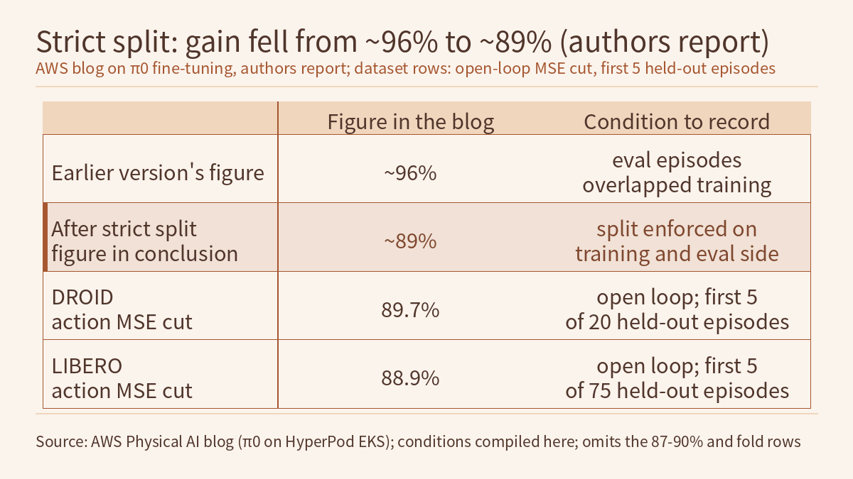
The video for episode 3.6 is about reading the frontier. When a number is inflated, it is usually not fraud; the measures do not line up, for example evaluation data mixed into the training set, a peak presented as the norm, or simulation taken for a real robot. For every paper, first run a checklist: who says it, what measure, how the data was split, whether the numbers add up, peak or typical, and whether the sample is big enough. Then go back to the original and copy a sentence that directly supports the number. The video’s examples come from two public sources: AWS’s engineering blog post on fine-tuning π0 on SageMaker HyperPod EKS, and the arXiv preprint Beyond Binary Success (2603.13616). This page is the reading and exercises for the episode. It does not repeat the transcript; it does three things the video concludes without working through. It takes the several “about 90%” figures in that one blog post and matches each to its metric and baseline, converting between percentage reductions and fold changes to see which sentence supports which number. It counts the training and held-out episodes from the blog’s split table, works out how much of the held-out set N=5 covers, and finds the layer the source leaves unstated. And it puts the 70% and 50% in the paper’s abstract back on their own baselines, showing why two “up to” figures cannot be chained. One rule runs through the whole page: record a number together with its metric, baseline, data split and sample size; if any of these is missing, the number cannot be retold on its own.
The video, transcript and sources for this lesson are at the top of this page; the season plan is in the course outline. The previous lesson, Physical AI Lab 3.5: Fine-Tuning GR00T in Practice — Checking the Fine-Tuning Command and the Modality Wiring Item by Item, Then Using a CPU Stand-In to Separate Open-Loop Error from Closed-Loop Success, ended by asking: how do you tell whether these success rates and improvements are real or overstated? This lesson picks up that question. How far apart open-loop error and closed-loop success are was worked out with a stand-in experiment in 3.5; the same AWS blog post’s “under 200 ms, re-planning at about 5 Hz” was used in Physical AI Lab 3.4: Long-Horizon Tasks — Working Out Per-Step and Whole-Chain Success by Hand, Seeing Which Quantity Progress Memory Changes, Then Reviewing a Routing Ablation That Swaps Only the Upper Layer. The three O/R/M levels, the point that “up to” does not mean “typical”, and the point that the 70% is saved evaluation effort rather than a success rate were covered and practised in Physical AI Lab 0.6: How to Judge Robot News — Tracing Each Question Back to a Sentence in the Source. Paired comparisons and intervals were worked out in Physical AI Lab 1.8: Evaluation — Splitting a “Net Gain of 2” into a Paired Table, Then Checking the Failure Labels and Random Seeds and Physical AI Lab 2.8: Reproducible Evaluation — Working Out Wald and Wilson Intervals by Hand, Sizing a Run from 1/√n, Then Bounding the Failure Rate after Zero Failures. The paper’s method itself is introduced in this site’s radar article Frontier Radar | Beyond Binary Success: sequential tests that separate robot policies with fewer real-world rollouts. This lesson does not repeat any of that; it covers only the three steps an L3 reader takes when checking a source: match the metrics, count the split, and separate the baselines. The next episode, 4.1, is about bodies and supply chains: actuators, BOMs and cost curves.
The public quiz’s 5 questions come with full explanations. Signed-in readers can do three exercises: reconcile the six groups of figures in the AWS blog post into one check record, converting reductions and fold changes, and review four fictional retellings; check the blog’s split table and the coverage of N=5, then rewrite the split for a fictional dataset whose episode count does not match; and review a fictional retelling of the paper, putting 70% and 50% back on their own baselines and rewriting it. Each comes with a step-by-step worked solution, common mistakes and a 20-point rubric.
1. The level of each of the three sources, and the fields a check record needs
The AWS blog post (Fine-Tuning π0 (Pi-Zero) for robotic manipulation on Amazon SageMaker HyperPod EKS) is AWS’s report of one fine-tuning experiment of its own. π0 is Physical Intelligence’s 3-billion-parameter flow-matching VLA; the post fine-tunes it on two datasets: lerobot/droid_100, recorded on a real Franka arm, and lerobot/libero_10, from a simulated Franka Panda arm. In this course’s grading it is level O, and all the numbers below are reported by the authors. This site did not run the pipeline.
Beyond Binary Success (arXiv 2603.13616) is by authors from the University of Pennsylvania, Toyota Research Institute and Princeton University. The paper proposes N-SCORE, a sequential comparison method based on safe, anytime-valid inference (SAVI): evaluation can stop early once enough evidence has accumulated, and the metric can be binary success or a bounded continuous quantity such as partial credit, reward or trajectory smoothness. It is a preprint, level R in this course’s grading; everything below is likewise reported by the authors, and this site has not reproduced it. This lesson read the arXiv HTML text from the abstract to the start of section IV, not the results sections or supplementary material.
The README of Physical AI Radar defines the three levels. The original, in Chinese, reads:
[O] 一手官方 · [R] 论文预印本 · [M] 媒体二手。厂商自报与同行评议不混为一谈。
That is: [O] official first-hand, [R] paper or preprint, [M] second-hand media; vendor self-reports and peer review are not treated as the same thing. The “how to read” section of the same README adds that R-level numbers are self-reported by the authors, and that even at level O you must tell “available on the platform” apart from “deployed by customers”. So the O on the AWS blog post means “AWS said it first-hand”, not “independently verified”.
The video says the output of a check is “number + one original sentence that directly supports it + evidence level + link”. An L3 reader needs a few more fields, because the problems found in the next three sections all sit in those fields. The table below is the record format this lesson suggests, not a rule from any source; the example is the DROID number in the blog post:
| Field | What to write | Example: the blog’s DROID number |
|---|---|---|
| Number | The value as written, with qualifiers such as “about” or “up to” | 89.7% |
| Quote | One sentence copied word for word, one per entry, never spliced | See the first quotation in section 2 |
| Metric and unit | What is measured; a reduction or a fold change | Reduction in action-prediction MSE |
| Baseline | Compared with what | The base checkpoint (lerobot/pi0_base) |
| Data and split | Which dataset; which episodes for training and for evaluation | lerobot/droid_100, training 0–79, held out 80–99 |
| Sample size | How many episodes and seeds were actually averaged | First 5 held-out episodes; the text read gives no seed count |
| Evaluation mode | Open or closed loop; simulation or real robot | Open loop, against recorded trajectories |
| Level, link, date checked | O / R / M, the source link, the day you opened the source | O, the AWS blog link, your own check date |
| Not stated in the source | The part retellers most often fill in | Closed-loop success rate, intervals, seed count |
The last field is the one most often dropped. People retelling a result tend to fill in what the source does not say, for instance writing a reduction in open-loop MSE as a success rate. Listing it separately tells you, the next time you cite the number, what you cannot say.
Sign in to keep reading: the rest of this lesson, its self-check questions and the answers.
Limitations
- The AWS blog post is level O, AWS’s report of one fine-tuning experiment of its own: ~96%, ~89%, 89.7%, 88.9%, 87-90%, 3.7×–5.6×, roughly 9×, the split table and N=5 are all reported by the authors. This site did not run the pipeline or check its repository. The text read is an excerpt of the post’s body, and it shows no seed count or confidence interval.
- Beyond Binary Success is a preprint, level R; 70%, 50%, 10–60 trials, over 4500 and 2000 rollouts, and the Type-1 error proof are reported by the authors, and this site has not reproduced them. This lesson read the text from the abstract to the start of section IV, not the results sections or supplementary material, so it does not know on which dataset and metric the upper bounds occurred. “The 50% baseline is STEP or a method of that kind” is this lesson’s inference.
- The radar’s O/R/M levels classify sources and remind you how much weight a sentence carries; they are not a judgement on whether a conclusion is correct.
- The following are this lesson’s calculations, summaries or suggestions: the conversions between reductions and fold changes, the coverages, the literal reading of the first five as 80–84 and 304–308, the record format in section 1, the comparison tables in sections 2 and 4, and the argument that 40% cannot be derived.
- R1–R4, toy_shelf, colleague K’s summary, the 60-trial and 50-trial plans, preprint P and method X are fictional. Open-loop error and paper calculations are not task success rates, and none of them is hardware safety validation.
Links
- Physical AI Lab: a physical AI course where every number can be checked (course outline)
- Physical AI Lab 3.5: Fine-Tuning GR00T in Practice — Checking the Fine-Tuning Command and the Modality Wiring Item by Item, Then Using a CPU Stand-In to Separate Open-Loop Error from Closed-Loop Success
- Physical AI Lab 3.4: Long-Horizon Tasks — Working Out Per-Step and Whole-Chain Success by Hand, Seeing Which Quantity Progress Memory Changes, Then Reviewing a Routing Ablation That Swaps Only the Upper Layer
- Physical AI Lab 0.6: How to Judge Robot News — Tracing Each Question Back to a Sentence in the Source
- Physical AI Lab 1.8: Evaluation — Splitting a “Net Gain of 2” into a Paired Table, Then Checking the Failure Labels and Random Seeds
- Physical AI Lab 2.8: Reproducible Evaluation — Working Out Wald and Wilson Intervals by Hand, Sizing a Run from 1/√n, Then Bounding the Failure Rate after Zero Failures
- Frontier Radar | Beyond Binary Success: sequential tests that separate robot policies with fewer real-world rollouts
- Physical AI Radar: an embodied AI morning brief with an evidence level on every item
- AWS: Fine-Tuning π0 (Pi-Zero) for robotic manipulation on Amazon SageMaker HyperPod EKS
- Beyond Binary Success: Sample-Efficient and Statistically Rigorous Robot Policy Comparison (arXiv 2603.13616)
- Physical AI Radar (GitHub, explanation of the O/R/M evidence levels)