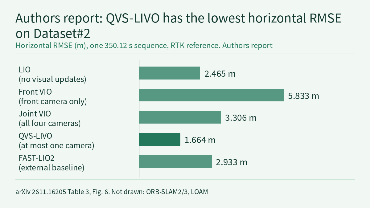
An off-road robot with four cameras cannot trust every camera at every moment. Canopy shade, sudden changes in light and a dropped stream can each degrade one viewing direction, while a lidar in sparse structure may leave some pose directions weakly constrained. In the preprint QVS-LIVO RiskMap (arXiv 2611.16205), Zihan Pan and colleagues at the State Key Laboratory of Robotic Technology and System, Harbin Institute of Technology, separate the two uses of the cameras. State estimation admits at most one camera to each photometric correction and keeps the lidar–inertial result when no view qualifies or the correction fails its checks; semantic risk mapping uses every available view. The authors report a horizontal RMSE of 1.664 m on the 350.12 s Dataset#2, against 3.306 m for Joint VIO, which fuses all four cameras. All numbers below are reported by the authors [R]; this site has not run their code.
Platform and problem
The platform is an AgileX Scout Mini chassis carrying an Airy lidar with a built-in IMU and four Intel RealSense D435i cameras facing front, left, rear and right. Each camera has a 69° horizontal field of view; the four views do not overlap and leave gaps between them. Four support pillars also cut the lidar’s horizontal coverage into four 86° sectors. The cameras have no hardware synchronisation and are paired by source timestamp within a soft-synchronisation window. Onboard computing is an NVIDIA Jetson AGX Orin. A separate C430i RTK-GNSS/INS logs reference positions at 1 Hz for offline evaluation of the horizontal trajectory only; neither localisation nor mapping uses it.
The estimator builds on the lidar–inertial estimation and direct photometric update framework of FAST-LIVO2. The paper starts from this observation: a view with good image quality may only reinforce directions the lidar already constrains well, and a view that would fill a weak lidar direction may be unreliable. Feeding degraded views or images with wrong time association into the pose update costs computation and can pull the pose off. Mapping needs something else: a camera not chosen for localisation can still see obstacles outside the main field of view.
Localisation front end: choosing the one camera
Each cycle runs the steps below; the parameters are the experimental settings in Table 2 of the paper:
- Batching: by source timestamp, at most one image per camera is taken within [t0, t0 + 2Δs], with soft-synchronisation tolerance Δs = 20 ms.
- Read-only pretracking: every view computes residuals and pose Jacobians on the same lidar–inertial posterior without changing the posterior or the visual map, which gives a common reference for comparison. The pretracking budget is 240 points in total, at most 60 per view.
- Health h: seven metrics are each normalised to [0, 1] and averaged with weights of 25% for tracked point count, 15% for tracking ratio, 20% for photometric residual, 10% for image coverage, 10% for the overexposed-pixel ratio, 10% for the dark-pixel ratio and 10% for mean gradient.
- Complementarity c: the normalised lidar information matrix is eigen-decomposed, directions whose information falls below a threshold (5% of the largest eigenvalue) get larger weights, and the score measures how much of the view’s visual information falls along those weak directions. Within the batch of eligible views, c is divided by its maximum to give c̃ ∈ [0, 1]. The combined score is q = h × (1 + γc̃), with γ = 2.
- Channel states: each camera is in one of four states: Healthy, Degraded, Isolated or Probation. Persistent low health or tracking failure marks degradation, and a hard image fault isolates the channel at once. A recovering channel enters Probation and becomes eligible again only after the required count of healthy observations and recovery time; an interrupted recovery sends it back to Isolated.
- Switching hysteresis: while the current view stays eligible, a challenger’s q must exceed 1.10 times the current view’s score for 3 consecutive valid cycles (margin m = 0.10) before a switch. If the current view becomes ineligible, reselection is immediate.
- Checks before commit: the correction is rejected if the batch, camera, timestamps or posterior generation differ from those used in evaluation. Lower health inflates the visual covariance more, by the factor κ = min(10, 1 / max(h, 0.10)). After solving, residuals, pose increment and the numerical validity of the normal equations are checked. If any check fails, the posterior is kept and the correction discarded.
A set of numbers invented by this site (not from the paper) shows how the combined score ranks views. The currently selected camera A has h = 0.80 and c̃ = 0.25, so q = 0.80 × 1.5 = 1.20. Challenger B has a worse image but covers the weak lidar direction: h = 0.60, c̃ = 1.00, q = 0.60 × 3 = 1.80. 1.80 exceeds 1.10 × 1.20 = 1.32, but B must stay ahead for 3 consecutive valid cycles before it is selected. Once it is, κ = 1 / 0.60 ≈ 1.67, so its photometric residuals are down-weighted according to its health. With γ = 2, complementarity can at most triple a view’s score, which is why a view with lower health but strong complementarity can win.
Risk mapping: geometry sets the ceiling, semantics make a bounded correction
The mapping branch is independent of the localisation choice and uses every available camera. The semantic network TraverNet adapts the Ultralytics YOLO26s dense semantic model to four classes: grass, road, tree and other. Semantic results are paired with point clouds by source timestamp (0.5 s window) and projected onto a world-anchored 2.5D grid. When several views cover a point, the one with the smallest optical depth is used, and semantic evidence decays with a 5 s half-life.
Geometric risk is a continuous value built from slope, step height and roughness. A cell with above-ground structure inside the vehicle’s passage band takes maximum risk regardless of its semantic class. Semantics may correct only unoccupied cells, with a weight capped at 0.35, so geometry keeps the larger continuous weight. Confirmation takes two paths. A hard obstacle that meets the occupancy-confidence threshold is confirmed at once. A candidate raised by slope or step needs at least 2 connected cells and at least 2 votes in the 3 latest evaluations. High-confidence low-risk semantics or previously traversed footprints can veto a candidate vote, but they cannot revoke a hard obstacle or create confirmed high risk on their own. Cells without valid geometric observations stay “unknown” instead of being treated as zero risk. There are three outputs: a Local Risk BEV, a global 2.5D Semantic–Terrain Risk Map and Obstacle Instance Voxels.
The authors report a four-class mIoU for TraverNet of 82.29% on 11 local validation images and 70.37% on 962 GOOSE validation images. In the Dataset#1 scene statistics, the mean risk for road, grass, other and tree is 0.159, 0.287, 0.660 and 0.741. The text we read gives no quantitative evaluation of the risk map against traversability ground truth.
Localisation and fault results reported by the authors
The two field sequences, Dataset#1 (178.78 s) and Dataset#2 (350.12 s), contain both off-road terrain and paved surfaces, with the reference trajectory from the C430i. All four ways of using vision are based on FAST-LIVO2: LIO disables visual updates; Front VIO uses only the front camera, the original FAST-LIVO2 configuration; Joint VIO fuses all four; QVS-LIVO selects at most one at a time. η_V is the fraction of time with valid visual tracking. For Joint VIO a moment counts as valid if any camera is valid; for QVS-LIVO only the selected camera counts.
| Method | Dataset#1 RMSE (m) | Dataset#1 η_V (%) | Dataset#2 RMSE (m) | Dataset#2 η_V (%) |
|---|---|---|---|---|
| LIO | 1.042 | – | 2.465 | – |
| Front VIO | 1.222 | 44.9 | 5.833 | 64.9 |
| Joint VIO | 1.190 | 90.0 | 3.306 | 96.0 |
| QVS-LIVO | 0.910 | 86.6 | 1.664 | 95.3 |
The row to look at is Joint VIO. On Dataset#2 it has the highest visual-tracking fraction (96.0%), yet its horizontal RMSE is 3.306 m, higher than LIO, which uses no vision at all (2.465 m). The authors read this as tracking availability not translating into better pose constraints: degraded or redundant views give the lidar–inertial posterior little help. For coloured maps, QVS-LIVO maps with all four cameras and keeps 2.24 and 3.02 times as many valid coloured voxels as Front VIO on Dataset#1 and Dataset#2 respectively, slightly fewer than Joint VIO, which also colours from four views.
Against external baselines, FAST-LIO2 (the vehicle-compatible variant used in the paper) scores 0.987 m and 2.933 m on the two sequences, and QVS-LIVO is 7.8% and 43.3% lower. ORB-SLAM2 scores 1.197 m and 4.425 m, ORB-SLAM3 1.323 m and 4.011 m, and LOAM 5.682 m and 7.036 m.
The fault experiment runs on Dataset#2 only. Within source time [105, 120) s, one fault is applied to one of the front, left, rear or right cameras while all other inputs stay unchanged; three fault types times four cameras give 12 configurations.
- Dropout: the evaluated Joint VIO implementation built up a processing backlog and terminated its trajectory in all four configurations. Front-only FAST-LIVO2 rose from 5.83 m to 14.40 m under front-camera dropout, and ARTI-VIO from 7.27 m to 17.42–29.24 m. QVS-LIVO scored 1.76–2.21 m.
- Black frames: Joint VIO scored 2.08–2.39 m. QVS-LIVO scored 1.75 m, 1.86 m and 1.94 m for front, rear and right camera faults, and both methods scored 2.09 m for the left camera.
- Timestamp shift of +60 ms: front-camera ORB-SLAM2 rose from 4.43 m to 58.70 m. Joint VIO scored 2.14–3.25 m and QVS-LIVO 1.54–2.23 m; for the left camera Joint VIO was slightly lower (2.14 m against 2.23 m).
QVS-LIVO produced complete trajectories in all 12 configurations, with horizontal RMSE of 1.54–2.23 m, 23.9%–47.4% below the 2.93 m normal-run result of the camera-independent FAST-LIO2. Note that the lowest fault-case value, 1.54 m, is below QVS-LIVO’s own normal-input 1.664 m. This site infers that this may reflect variation between single runs, or the fault may have changed which view was selected; the paper reports no repeated runs or spread, so differences of a few tenths of a metre between fault configurations should not be read as a firm ordering.
Onboard runtime
On the AGX Orin, the Local Risk BEV is output at 9.94 Hz with a median processing time of 32.4 ms and a P95 of 37.9 ms (30 s observation window). The global map runs at 2.00 Hz with a median of 486.4 ms and a P95 of 516.1 ms (180 s observation window). Table 2 of the paper configures the two publication rates at about 10 Hz and about 2 Hz, so 9.94 Hz and 2.00 Hz are output rates reached at the configured pace and do not show the processing-capacity ceiling. The global map’s P95 already exceeds the 500 ms period of 2 Hz (this site’s calculation), and the text we read does not say how the pipeline handles those overruns. All of these timings are for mapping; the text we read gives no separate per-cycle time for the localisation front end on the Orin.
How this relates to the course on this site
Physical AI Lab 1.3 explains that each sensor sees one side of the world, that no sensor is perfect and that sensors need to check one another. This paper gives one concrete way to do it: score each camera on a shared lidar–inertial posterior first, then decide whether it may change the pose, and fall back to the original result if it does not qualify. For what frequency, median and P95 each tell you, and the difference between a configured rate and a capacity ceiling, see Physical AI Lab 2.6. The paper reports no repeated runs for the 12 fault configurations; how to read results condition by condition and why the number of repeats matters is covered in Physical AI Lab 1.8. The full season is in the course outline.
Limitations
- This is an arXiv preprint; all numbers are reported by the authors [R] and this site has not reproduced them. The paper says its code and related resources are public; this site has not checked that repository.
- The evaluation covers one platform and two sequences (178.78 s and 350.12 s), with a 1 Hz RTK-GNSS/INS reference and only horizontal error. The paper reports no repeated runs, confidence intervals or spread.
- Faults were injected into one camera at a time, within a 15 s interval of Dataset#2 only; simultaneous faults in several cameras and longer degradation are not covered. The paper limits the Joint VIO termination under dropout to “the evaluated Joint VIO implementation”; it does not extend to every joint-fusion method.
- For the risk map, the paper gives semantic-segmentation mIoU and mean risk per class; the text we read has no traversability ground truth or navigation results. The local semantic validation set has only 11 images.
- The text available to this site breaks off partway through the discussion section, so we have not read the authors’ own limitations section.
- The numbers for cameras A and B are a teaching example invented by this site, not results from the paper. This is an evaluation on field data and offline replay, not a hardware safety validation.
Links
- QVS-LIVO RiskMap: Health- and Information-Aware View Selection for Multi-Camera LIVO and Off-Road Risk Mapping (arXiv 2611.16205)
- Full paper in HTML
- Physical AI Lab 1.3: Sensors — Working Out Pixels, Depth Range and Grip Force for One Cup
- Physical AI Lab 2.6: To the Edge — Working Out the Control-Rate Ceiling from a Latency Log, Telling Whether Quantization Saves Size or Time, Then Sizing an Action Chunk
- Physical AI Lab 1.8: Evaluation — Splitting a “Net Gain of 2” into a Paired Table, Then Checking the Failure Labels and Random Seeds
- Physical AI Lab: a physical AI course where every number can be checked