UAV-Flow++ (arXiv 2611.17163, 2026-11-12) is a preprint led by Beihang University, with co-authors from the National University of Singapore and MMLab at The Chinese University of Hong Kong. It studies this drone problem: after a short instruction such as “pass that tree on the left”, a policy turns the onboard camera view and the current state directly into continuous flight actions and flies a short-range maneuver. The authors argue that language-guided UAV research has mostly addressed long-distance route planning, and that short-range maneuvers relative to objects have received little study. The paper releases 30,692 real-world demonstrations flown by professional pilots, a closed-loop simulation suite with automatic scoring, UAV-Flow-Sim, and a policy, FlowVLA, that is first trained by imitation and then post-trained with reinforcement learning in simulation. The authors report that on 273 held-out simulation episodes, FlowVLA reaches a 75.58% success rate after pretraining and 93.16% after TGRPO post-training. All numbers below are author-reported [R]; this site has not run the authors’ code or downloaded the data.
The task: one instruction, one short maneuver
The authors call the task Flying-on-a-Word (Flow). At each time step the policy receives three inputs: a natural-language instruction, the drone’s 6-DoF state in a local frame whose origin is the start of the episode, and the onboard first-person image. It outputs a target pose or a “position + yaw” command in that local frame, which can then be mapped to a specific platform’s flight controller. The task tests two abilities. The first is understanding the intended motion, such as translating in a direction, rotating by an angle, ascending, hovering or landing. The second is grounding the instruction’s spatial references in the image, such as approaching a car, passing an object on a given side or stopping next to a landmark. Instructions therefore come in two groups: primitive motion commands and object-interactive commands.
Table 1 of the paper lists earlier language-guided UAV benchmarks side by side: AVDN, AerialVLN, CityNav, OpenUAV, OpenFly, IndoorUAV and HUGE-Bench all take their data from simulation, and most target long-horizon or goal-directed navigation. UAV-Flow combines simulation and real flights, uses continuous 6-DoF actions, has about 40K trajectories and works at the granularity of short-range execution. The authors write that most UAV-Flow trajectories are shorter than 20 meters. The paper extends the authors’ conference version, UAVFlow, adding automatic task-level scoring, mixed-data pretraining followed by online RL post-training, and a fuller set of comparisons and ablations.
The data: real demonstrations and simulated trajectories
The real data were collected on three university campuses covering 5.02 km², with pedestrians, vehicles, vegetation, buildings, roads, open spaces and landmarks. Certified pilots, each with more than 800 hours of flight experience, flew commercial platforms such as the DJI Mavic 3T RTK with a 4K camera and an RTK GPS module, giving centimeter-level trajectory accuracy. Pilots executed instructions using only the onboard view, so the recorded images match what a deployed policy sees. Each instruction was flown from several starting positions and headings, so one intent yields several different trajectories. Video and flight logs were aligned by timestamp, with the 6-DoF state interpolated for every frame and then converted to a local frame centered at the start, with orientation relative to the initial heading, sampled at 5 Hz. Annotators first removed clips with ambiguous behavior, unsafe execution, unclear spatial relations or inconsistent semantics, then assigned canonical labels from a fixed command set; a large language model paraphrased these into open-vocabulary commands. The result is 30,692 trajectories in 8 major motion categories.
UAV-Flow-Sim is built in a campus scene, rendered and controlled through UnrealCV with a “position + yaw” interface, and contains static landmarks plus interactive objects such as people, vehicles and quadruped robots. Of its 10,109 trajectories, some were flown by human pilots, while fixed maneuvers were generated by rule-based scripts that use privileged simulator information (drone state and object positions). The two action distributions differ (Table 2 of the paper): in the real data, “approach” and “pass through” are the most common, at 28.1% and 28.4%; in simulation, “shift” and “approach” lead, at 29.4% and 25.6%. The real data contain 3.2k hovering trajectories; the simulated data contain none.
Pretraining does not use all the real data. The authors selected 9,766 real trajectories for task balance and trajectory quality and added the 10,109 simulated ones, for 19,875 trajectories and 946,607 frames. By this site’s calculation that is about a third of the real data (9,766 ÷ 30,692 ≈ 0.32).
How the simulator scores an episode
In closed-loop evaluation the simulator passes the current image and state to the policy at each step, executes the action it returns and sends back the next frame. An episode ends on task completion, collision, a safety violation or when the step limit runs out, and the simulator records the full trajectory, the terminal state, object relations and collision events. Each episode receives a completion score for its task type k, C_k = C_proc + C_goal, between 0 and 1. The first term scores the maneuver itself, for example whether a “pass through” episode actually passed the specified object or region; the second scores the terminal state, for example whether the drone stopped at the target position. Distance and angle terms use a clipped interval score Φ(d, Δ, w) = max(0, w − 0.1⌈d/Δ⌉), where d is the error, Δ is the error interval for each 0.1-point deduction and w is the term’s maximum.
The paper text read here does not give w or Δ for each task. One hypothetical worked case: with w = 0.5, Δ = 0.5 m and a terminal error d = 1.2 m, ⌈1.2/0.5⌉ = ⌈2.4⌉ = 3, so the term scores 0.5 − 0.3 = 0.2. Above 2.0 m of error the term is 0, and any error greater than 0 costs at least 0.1. These numbers only illustrate the formula; they are not the paper’s settings.
The paper reports three metrics: success rate (SR; an episode counts as a success only when all applicable completion criteria are met), completion score (CS) and normalized dynamic time warping (NDTW, the similarity between the executed and reference trajectories, where each point combines position with the cosines of roll, yaw and pitch). The test set has 273 annotated episodes, each with an initial state, an instruction, a reference trajectory and completion criteria. Note that these test episodes use the same campus scene in which the simulated demonstrations were collected, and RL post-training also runs in this simulator. “Held-out” applies at the episode level; the scene does not change.
FlowVLA and TGRPO: imitation first, then weighting by the group’s reward distribution
FlowVLA consists of a pretrained Qwen3-VL backbone and a lightweight discrete action head. Its inputs are the episode’s first image, the current image, and the state (x, y, z, yaw) written as text and appended to the instruction. The model predicts 10 “position + yaw” steps at a time, with 256 bins for each of the 4 dimensions; at the 5 Hz sampling rate one action chunk covers 2 seconds. Pretraining fine-tunes the VLM with LoRA and trains the action head with cross-entropy for 80,000 steps on eight NVIDIA L40 GPUs.
The authors’ reason for post-training is that imitation covers only states near expert trajectories; deviations during closed-loop execution carry the policy outside the demonstration distribution, and errors compound. Physical AI Lab 1.6 works through how such an error rolls out of the demonstrations’ coverage. RL runs in the SimpleVLA-RL framework and trains only four task types, “pass”, “rotate”, “land” and “approach”, with 204 training trajectories per task and 90 policy updates in total. Each iteration samples 8 closed-loop rollouts on each of 16 parallel task configurations (128 in all) at temperature 1.6, with at most 100 simulator interactions per rollout. The reward is the completion score at the end of the episode, and evaluation uses greedy decoding.
Standard GRPO takes the group reward minus its mean, divided by its standard deviation, as the advantage. TGRPO adopts the threshold-based weighting of TailRL: sort the group rewards as r(1) ≤ … ≤ r(G) with r(0) = 0, compute the weight ω(r(i)) = Σ_{ℓ=1..i} (r(ℓ) − r(ℓ−1)) / (G − ℓ + 1), then subtract the group mean and multiply by the group size G to get the task advantage. The denominator is the number of trajectories whose reward exceeds that segment, so reward intervals that fewer trajectories reach get more weight. A group-centered KL penalty against the reference policy is then subtracted, and GRPO’s clipped objective is kept.
A hypothetical group shows the difference (G = 4, evenly spaced rewards, KL term left out):
| Trajectory | Reward (completion) | GRPO advantage (population std 0.224) | TGRPO task advantage |
|---|---|---|---|
| a | 0.4 | −1.34 | −0.60 |
| b | 0.6 | −0.45 | −0.33 |
| c | 0.8 | +0.45 | +0.07 |
| d | 1.0 | +1.34 | +0.87 |
The TGRPO column: ω is 0.4/4 = 0.10, then 0.10 + 0.2/3 ≈ 0.17, 0.17 + 0.2/2 ≈ 0.27 and 0.27 + 0.2/1 ≈ 0.47; the mean is 0.25, and subtracting the mean from each and multiplying by 4 gives the values in the table. GRPO’s advantages are symmetric about the mean, with either the population or the sample standard deviation. Under TGRPO, with the same 0.2 reward step, the advantage gap between c and d is 0.80 while the gap between a and b is only about 0.27, and c, whose reward is above the group mean (0.7), gets only a small positive advantage. This is what the authors mean by reinforcing rare high-reward trajectories more strongly. The table is this site’s exercise using the paper’s formula, not data from the paper. For how to read evidence on RL post-training in general, see Physical AI Lab 3.3.
Results: which comparisons in Table 3 share conditions
The overall results in Table 3 of the paper (273 test episodes, mean of three evaluation runs; only the three FlowVLA rows report a standard deviation):
| Method | Training data | Overall SR (%) | Overall NDTW |
|---|---|---|---|
| TravelUAV | Simulated demonstrations | 56.78 | 0.237 |
| OpenVLA-UAV | Simulated demonstrations | 53.85 | 0.345 |
| π0-UAV | Simulated demonstrations | 68.86 | 0.431 |
| MemoryVLA-UAV | Simulated demonstrations | 62.64 | 0.342 |
| π0.5-UAV | Simulated demonstrations | 66.67 | 0.398 |
| FlowVLA (pretrained) | Real + simulated demonstrations | 75.58 ± 1.12 | 0.402 ± 0.006 |
| FlowVLA-GRPO | Same, plus RL post-training | 92.06 ± 0.56 | 0.434 ± 0.005 |
| FlowVLA-TGRPO | Same, plus RL post-training | 93.16 ± 0.42 | 0.424 ± 0.008 |
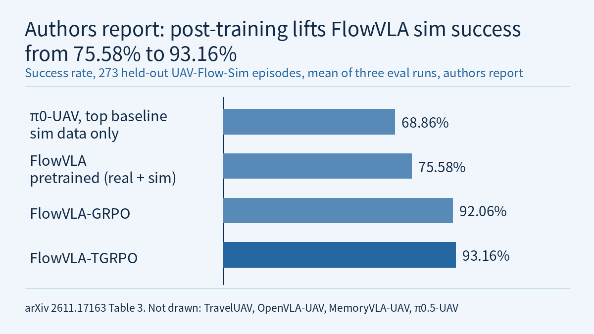
The chart in this article shows the overall success rate for four of these rows: π0-UAV 68.86%, pretrained FlowVLA 75.58%, FlowVLA-GRPO 92.06% and FlowVLA-TGRPO 93.16%. Several points in this table need to be read separately:
- Pretrained FlowVLA and the baselines use different data. All five baselines are trained by imitation on the same simulated demonstrations only (with LoRA fine-tuning of their VLM parts), their outputs are converted to local “position + yaw” commands, and the same simulator-side controller executes them; FlowVLA also uses real demonstrations. The 6.72-point lead the authors report therefore includes a data difference. In ablation Table 5, FlowVLA trained on simulated data alone reaches 73.14 ± 0.56%, which by this site’s calculation is still 4.28 points above π0-UAV, but that gap also includes differences in model architecture. Adding real demonstrations contributes 2.44 points (73.14% → 75.58%), while the evaluation itself is entirely in simulation.
- A higher success rate does not always mean higher trajectory similarity. Pretrained FlowVLA’s NDTW is 0.402, below π0-UAV’s 0.431. Per task, it reaches only 24.44% on “rotate”, where π0.5-UAV reaches 66.67%, and 55.00% on “pass”, below MemoryVLA-UAV’s 62.50%.
- The post-training gains compare runs from the same initialization, and they are far larger than the reported variation. From 75.58% to 92.06% for GRPO and 93.16% for TGRPO, the gains are 16.48 (this site’s calculation) and 17.58 points; both reach 100% on “rotate”. The large gains are on the four task types used in RL training, and testing takes place in the same simulated scene.
- TGRPO is only 1.10 points above GRPO. The standard deviations of TGRPO and GRPO are 0.42 and 0.56, from three evaluation runs. The paper text read here does not say what changes between the three evaluation runs under greedy decoding, and it reports no results across multiple training seeds. NDTW is higher for GRPO (0.434 vs 0.424). From Figure 6 the authors also report that TGRPO passes 90% overall SR after about 40 updates while GRPO needs about 80; the claim of better sample efficiency rests on this one set of training curves.
- Tasks left out of RL decline somewhat. The authors report that GRPO first drops on the remaining tasks and then returns close to the pretrained level, while TGRPO’s mean SR on the remaining tasks declines slightly late in training, by less than GDPO and DAPO. Other algorithms compared from the same initialization reach overall SRs of 82.91% for DAPO, 89.13% for GSPO and 89.87% for GDPO. The authors suggest that the late-stage degradation of DAPO and GSPO may be partly related to their lack of reference-policy KL regularization; the paper text read here does not test this separately.
- In the architecture ablations, replacing the discrete action head with a FAST head lowers SR to 64.10%; mixing features from all Qwen3-VL layers gives 76.19%, only 0.61 points above using the final layer alone, so the authors keep the final layer as the RL initialization.
Real-world deployment: inference on a ground station, skipping stale waypoints by measured delay
Onboard compute is limited, so VLA inference runs on a ground station. The drone sends images and state over a wireless link; the ground station produces an action chunk, converts it to waypoints and sends them back to the onboard flight controller. The drone keeps flying during inference, so the first waypoints of the returned chunk may already be outdated. The execution layer therefore uses the measured delay δ from image capture to command dispatch and the waypoint execution frequency f_c to skip the first m = min(H − 1, ⌈δ·f_c⌉) waypoints.
The paper text read here gives no measured values for δ or f_c. With hypothetical values: H = 10 (the paper’s setting); if f_c is 5 Hz and δ = 0.35 s, then ⌈1.75⌉ = 2, so the first 2 waypoints are skipped and execution starts at the 3rd. If δ = 2.5 s, ⌈12.5⌉ = 13 is capped at H − 1 = 9, leaving only the last waypoint. At 5 Hz a chunk covers only 2 seconds, so once the delay approaches that length, skipping waypoints can no longer compensate. Physical AI Lab 2.6 has a worked exercise on how chunk length relates to latency.
The real-world part is a qualitative demonstration. The outdoor sequences in Figure 7 use π0-UAV (passing a tree on the left, approaching the right side of a sign), and the indoor sequences in Figure 8 use FlowVLA (orbiting a tree clockwise, passing a sign on the left). The paper text read here reports no number of real flights or success rate; the abstract’s “robust execution” and the body’s statement that the flights substantiate the simulation results are the authors’ descriptions. In the conclusion the authors acknowledge that high-rate closed-loop control currently depends on ground-station compute and wireless communication, which brings latency risks and limits onboard autonomy; they plan model compression and onboard inference. This site has covered another drone approach before: event-camera quadrotor obstacle avoidance, where the policy maps event frames straight to acceleration and no language instruction is involved.
Limitations
- This is an arXiv preprint, and every number is author-reported [R]. This site has not run the code, downloaded the data or checked the tables. The HTML text read here ends at the conclusion; there may be appendices that were not read.
- All closed-loop success rates come from the same campus scene in UAV-Flow-Sim, where RL post-training also took place. There is no quantitative success rate in a different scene or on real hardware.
- The baselines are trained only on simulated demonstrations while FlowVLA also uses real ones, so the pretraining comparison does not use the same data.
- TGRPO’s 1.10-point lead over GRPO comes from statistics over three evaluation runs; the paper text read here has no results across training seeds, and NDTW points the other way.
- RL covers only four task types, and the authors report a small late-stage decline on the remaining tasks.
- The real flights are qualitative demonstrations, and the outdoor ones use the baseline π0-UAV. Neither the simulation results nor these demonstrations are flight-safety validation, and they do not show usability on other platforms, in other airspace or in other weather.
- The two hypothetical calculations (the clipped interval score and the number of skipped waypoints) and the small TGRPO advantage table are this site’s exercises, not data from the paper.
Links
- UAV-Flow++: A Unified Suite for Benchmarking and Learning Language-Guided UAV Flight (arXiv 2611.17163)
- Full paper in HTML
- Project page (as listed in the paper)
- Code repository buaa-colalab/UAV-Flow (as listed in the paper)
- Hugging Face dataset wangxiangyu0814/UAV-Flow (as listed in the paper)
- Physical AI Lab: a physical AI course where every number can be checked (course outline)
- Physical AI Lab 1.6: Imitation Learning — Working Out How an Error Rolls Out of the Demonstrations’ Coverage, Then Putting the ACT, Diffusion Policy and Data Scaling Numbers Back in Their Own Conditions
- Physical AI Lab 2.6: To the Edge — Working Out the Control-Rate Ceiling from a Latency Log, Telling Whether Quantization Saves Size or Time, Then Sizing an Action Chunk
- Physical AI Lab 3.3: RL Post-Training — Putting HIL-SERL’s “2x” and RECAP’s “Doubled Throughput” Back in Their Conditions, Then Recomputing the Paired Interval over Three Seeds
- Frontier Radar | Event-camera quadrotor obstacle avoidance: a CUDA event simulator inside differentiable simulation, with a policy that maps event frames straight to acceleration