
Lesson video
Narration is AI-generated. Video chapters, transcript and sources
Transcript
Transcript
UNIT-01 asks
A robot policy reports a success rate of eighty-four percent. Do you really dare to trust that number? Last time, we built a safety filter. This time we ask: how do you prove it really works? The answer is repeated trials, and confidence intervals.
The lie of a single success rate
Let's run an experiment, all simulated in this episode's notebook. Suppose the true success rate is exactly seventy percent. We let it run, and see what gets reported. Run one round, and count the successes. It comes out at exactly seventy percent. Looks pretty accurate. First, to be clear, a success rate is just a ratio. Successes, divided by attempts. But the simpler the number, the easier it is to misread. But what if you run another round? Change only the random seed, and the number moves. This round, maybe only sixty percent. Don't rush to blame this policy. It may really be a seventy percent policy. This time, it was just a bit unlucky. Worse is cherry-picking. Run many rounds, and report only the best one. A number like that is fooling yourself. Same policy, twelve rounds. The highest and lowest can be far apart. It's all luck, swinging back and forth. This isn't made up; a paper has tested it. Ten runs of the same setup, changing only the seeds. Split into two groups, and the conclusions can differ significantly. So if you only run once, what you see might just be luck! Think of flipping a coin. Flip it ten times, and five heads, five tails is normal. But seven heads and three tails is nothing strange either. Here's the pattern. The fewer the samples, the wilder the randomness. With more samples, it slowly settles down.
Give the success rate an interval
So don't report just one number. Give it an interval. Say clearly: roughly where does the true success rate fall? The most common method is called the Wald interval. It's the textbook's normal approximation. But it hides a big flaw. A statistics paper points out that for Wald, the textbook interval, coverage is persistently too low. Its recommendation: for small samples, use the Wilson interval instead. How does the Wilson interval work? It pulls the observed success rate gently toward the middle. The fewer the samples, the more it pulls. How absurd does it get? If all ten attempts succeed, Wald says the success rate is one hundred percent. And the interval's width is zero. That's clearly absurd. Ten out of ten, and you'd claim it will never fail? Wilson isn't that naive. Why is coverage too low for Wald? The normal approximation is especially poor with few samples and an extreme rate. But even with larger samples, its coverage swings up and down. The interval tells you something else. When comparing two policies, if their intervals overlap a lot, you can't call a winner yet. If they don't overlap at all, the gap is solid. So when you read a leaderboard, don't just stare at first place. Check how much their intervals overlap. For a rigorous comparison, compute an interval for the difference, or run a test. There's another general method, called the bootstrap. One paper resamples the results ten thousand times to compute its intervals. There are several ways to compute it. The simplest takes the middle range. The bootstrap's advantage is that it assumes no distribution or formula. But it treats the sample as if it were the population. With very few runs or an extreme rate, it breaks down too. So which one to trust? For small-sample success rates, prefer Wilson. With more samples and a complex statistic, use the bootstrap. So the interval isn't decoration! It shows how uncertain this number is.
How many runs?
So how many runs do you need? First, a rule. The interval's width shrinks slowly, roughly with the square root of n. That rule actually stings. To cut the uncertainty in half, you need four times the samples. Eight or ten runs won't be enough. If you want a decent interval, plan for a much bigger sample. Real-robot evaluation is even more precious. Every trial means really moving the robot. So samples are often painfully few. Look at it another way. The longer you watch, the more confidently you can say it really does rarely fail. There's another counter-intuitive trap. Here's an example from this episode's notebook. Suppose last episode's safety filter is tested one hundred times without a single failure. That still doesn't mean its success rate is one hundred percent. The fewer the samples, the looser this upper bound. Zero failures only means you haven't run into one yet. Not that it can't fail. So zero failures doesn't mean zero risk! You just haven't tried enough. So when you report a success rate, report three things with it. How many runs, which interval, and how wide. Don't leave any out. Report the random seeds too. That way, others can rerun your results exactly. The interval also tells you when you have enough samples. Don't just keep running blindly. The easiest thing to forget: define success and failure clearly first. Change the criterion, and every number changes. Be clear about the test setting, too. Where it was tested, how hard it was, whether the easy cases were picked. Change the setting, and the success rate means something else. Open the notebook and follow along. Evaluate the same policy over many rounds. Watch how those success rates spread out. Then draw a coverage curve. The line for Wald, you'll see, drops clearly below ninety-five percent. Wilson stays close to it, occasionally dipping slightly below. Finally, plot the interval's half-width against the sample size. You'll see for yourself how it slowly narrows with the square root of n. So the honesty of an evaluation lives in this interval! Let's recap. One, reporting a single success rate misleads; give an interval. Two, don't use Wald, the textbook interval; for small samples, use Wilson. The bootstrap suits larger samples and complex statistics. Three, fewer samples mean wider intervals, and zero failures isn't zero risk. Evaluation isn't about a pretty number. It's about knowing how sure you are! Now we know how sure a success rate is. And that big model that sees, thinks and acts: what does it look like inside? See you next time!
Evidence and sources
Practice and self-check
- Interactive quiz5 questions, explained as you answer
- One-page summaryprintable; opens in a new tab
- Download the notebookszip in Chinese, English and Japanese; run in Jupyter or upload to Colab
The quiz is public and explains each answer as you go; answers to the guide's exercises are for signed-in members.
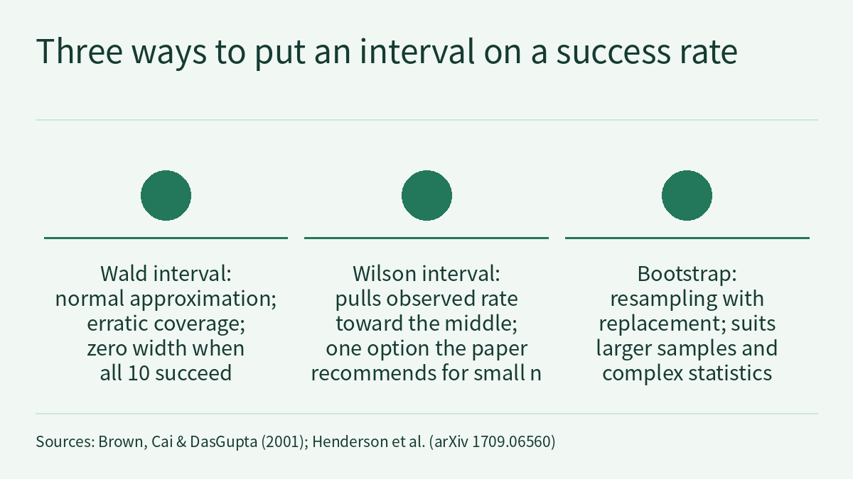
The video for episode 2.8 asks: a policy reports “84% success”; can you trust that number? The video makes three points. Reporting a single success rate misleads, because changing only the random seed makes the number jump, so you should give an interval. Don’t use the textbook Wald (normal-approximation) interval; for a small-sample success rate use the Wilson interval, and keep the bootstrap for larger samples and complex statistics. The width of the interval shrinks roughly as 1/√n, and zero failures does not mean zero risk. The three number cards in the video come from two public sources. In Henderson et al.’s Deep Reinforcement Learning that Matters (arXiv 1709.06560), ten runs of the same hyperparameters with only the random seed changed, split into two groups of five, can lead to statistically different conclusions; the same paper computes bootstrap 95% confidence bounds for average returns on several MuJoCo environments, with ten thousand resamples and the pivotal method. Brown, Cai and DasGupta’s Interval Estimation for a Binomial Proportion (Statistical Science, 2001) shows that the Wald interval’s coverage properties are chaotic and recommends the Wilson interval for small n. This page is the reading and exercises for the episode. It does not repeat the transcript. Instead it works out three things the video only states as conclusions: using a fictional 20-trial evaluation, it computes the Wald and Wilson intervals by hand to see why Wald can exceed 100% and has zero width when every trial succeeds; it uses the 1/√n rule to size an evaluation and derives how to bound the failure rate after zero failures; and it reads the real numbers in Henderson et al.’s Table 3 to see how intervals are used for comparison and why the bootstrap breaks down with very few samples. One rule runs through the whole page: an interval describes only its own set of trials, with their count, success criterion and setting, and a report must give the count, the type of interval and its width together.
The video, transcript and sources for this lesson are at the top of this page; the season plan is in the course outline. The previous lesson, Physical AI Lab 2.7: Safety Filters — Working Out One Control-Barrier-Function Correction by Hand, Then Choosing Its Loop and Its Safety Margin, ended by asking: how do we know this really works? This lesson answers. The original passage from Henderson et al. on “ten runs with only the seed changed, split into two groups” and its experimental conditions, along with how to pair success rates and classify failures, were covered and practised in Physical AI Lab 1.8: Evaluation — Splitting a “Net Gain of 2” into a Paired Table, Then Checking the Failure Labels and Random Seeds. This lesson does not repeat them. It covers only what is new in this episode: how to compute an interval, how many runs you need, how to report zero failures, and where the bootstrap applies. The next episode, 3.1, moves to L3 and takes apart a VLA’s vision encoder, language backbone and action head.
The public quiz’s 5 questions come with full explanations. Signed-in readers can do three exercises: compute Wald and Wilson intervals by hand for three fictional evaluations, plus the failure-rate upper bound after zero failures, and write the report sentences; set the number of trials and the time budget for an evaluation on a fictional real robot, then check the result with a Wilson interval; and review a fictional evaluation report that misuses the bootstrap, intervals and a stopping rule, then rewrite it. Each comes with a step-by-step solution, common mistakes and a 20-point rubric.
1. What each source says
Henderson et al., Deep Reinforcement Learning that Matters (arXiv 1709.06560; this lesson read HTML v1, submitted 2017-09-19). The authors are from McGill University and Microsoft Maluuba. The paper studies why reinforcement learning results are hard to reproduce, with policy gradient methods (TRPO, DDPG, PPO, ACKTR) on MuJoCo continuous-control tasks. Under this course’s grading it is level R, and everything below is author-reported; this site has not reproduced it. The “10 runs” number card corresponds to two sentences in the “Random Seeds and Trials” section, excerpted on their own:
We perform 10 experiment trials, for the same hyperparameter configuration, only varying the random seed across all 10 trials. We then split the trials into two sets of 5 and average these two groupings together.
The conditions of this experiment and the paper’s reading of it were covered in 1.8. Two other points in the same section matter here. The paper says that in recently reported results it is not uncommon to select the top N trials from among several, or to average over only a small number of trials (N < 5), and considers this potentially misleading. It also says that no specific number of trials can be given as a recommendation. The “cherry-picking” in the video’s first chapter refers to practices of this kind.
The “10,000 resamples” number card corresponds to the caption of Table 3:
Bootstrap mean and 95% confidence bounds for a subset of environment experiments. 10k bootstrap iterations and the pivotal method were used.
Table 3 gives the average return of four algorithms in four environments; each cell is the bootstrap mean, with the 95% confidence bounds in brackets. The general setup in the paper’s experiments section is 5 trials per evaluation, each with a different preset random seed, with all experiments using the same set of seeds. The caption of Table 3 does not separately state how many trials each cell uses. Section 4 uses the table below; here are the original numbers:
| Environment | DDPG | ACKTR | TRPO | PPO |
|---|---|---|---|---|
| HalfCheetah-v1 | 5037 (3664, 6574) | 3888 (2288, 5131) | 1254.5 (999, 1464) | 3043 (1920, 4165) |
| Hopper-v1 | 1632.1 (607, 2370) | 2546 (1875, 3217) | 2965 (2854, 3076) | 2715 (2589, 2847) |
| Walker2d-v1 | 1582 (901, 2174) | 2285 (1246, 3235) | 3072 (2957, 3183) | 2926 (2514, 3361) |
| Swimmer-v1 | 31 (21, 46) | 50 (42, 55) | 214 (141, 287) | 107 (101, 118) |
Brown, Cai and DasGupta, Interval Estimation for a Binomial Proportion (Statistical Science 16(2), 2001). This is a statistics journal paper, level R under this course’s grading; this lesson read its abstract. A binomial proportion is the proportion in data of the form “so many successes out of n”, and a success rate is exactly such a proportion. The “Wald→Wilson” number card corresponds to two sentences in the abstract, excerpted on their own:
We begin by showing that the chaotic coverage properties of the Wald interval are far more persistent than is appreciated. Furthermore, common textbook prescriptions regarding its safety are misleading and defective in several respects and cannot be trusted.
Based on this analysis, we recommend the Wilson interval or the equal-tailed Jeffreys prior interval for small n and the interval suggested in Agresti and Coull for larger n.
“Coverage” means this: if you repeat the evaluation and compute the interval the same way each time, it is the proportion of intervals that contain the true success rate. For a nominal 95% interval, coverage should be close to 95%. The abstract says the Wald interval’s coverage properties are chaotic, and more persistently so than is appreciated, and that textbook rules of thumb for when it is “safe” cannot be trusted.
| Number in the video | Source | Conditions in the original | What the original does not say | Level |
|---|---|---|---|---|
| 10 runs | Henderson et al., Random Seeds and Trials section | Same hyperparameters, only the random seed changed, 10 runs split into two groups of 5 and averaged; the subject is reinforcement learning training results | Not a robot success-rate evaluation; the paper says no specific number of trials can be recommended | R (author-reported) |
| 10,000 resamples | Henderson et al., caption of Table 3 | Bootstrap mean and 95% confidence bounds for average returns in a subset of environment experiments; 10k bootstrap iterations, pivotal method | The subject is return, not success rate; the parts read do not define the pivotal method, and the caption of Table 3 does not state the number of trials per cell | R (author-reported) |
| Wald→Wilson | Brown, Cai and DasGupta, abstract | Interval estimation for a binomial proportion; Wald’s coverage properties are chaotic; Wilson or equal-tailed Jeffreys recommended for small n, Agresti and Coull’s interval for larger n | The abstract gives no threshold for “small n” and does not write out the formulas | R (journal paper) |
When reading this table, note that Henderson et al. study the randomness of training, and their numbers are returns; Brown et al. study intervals for a binomial proportion, and their numbers are proportions like a success rate. The video puts the two in one episode because they answer the same question: how much uncertainty lies behind one number. The numbers from the two sources cannot be converted into each other.
Sign in to keep reading: the rest of this lesson, its self-check questions and the answers.
Limitations
- Henderson et al. (arXiv 1709.06560, HTML v1, submitted 2017-09-19) is level R and a preprint. This lesson read the abstract, the introduction, the experimental setup, Tables 1, 2 and 3 of the hyperparameter section, and the “Random Seeds and Trials” section up to the start of the caption of Figure 5; the ten runs split in two, the 10k-iteration pivotal bootstrap and the numbers in Table 3 are author-reported, and this site has not reproduced them. The parts read do not define the pivotal method, and the caption of Table 3 does not state the number of trials per cell.
- Brown, Cai and DasGupta (Statistical Science 16(2), 2001) is level R; this lesson read only the abstract. The Wald and Wilson formulas are the standard forms this lesson uses; the abstract does not write them out, and it gives no threshold for “small n”.
- The following are this lesson’s derivations, readings or advice: the reading of the Wilson centre as “pulled toward the middle”; the Wilson lower bound n/(n + z²) when every trial succeeds; the planning formula n ≈ z²·p(1−p)/E²; the zero-failure bound 1 − 0.05^(1/n) and the 3/n approximation; the half-width of the difference of two independent estimates; the derivation of bootstrap quantiles for 10/10 and 9/10; judgements such as “the pooled interval does not include differences between seeds” and “stopping on the conclusion is a variant of cherry-picking”; and the advice to fix the criterion, setting, seeds and trial count before starting.
- Policies X, Y, A, B, C and N, arm M, team Q, and all counts, successes, times, hours and per-seed results in sections 2 to 5 are fictional; example figures in the text such as 0.640, 0.722 and 9.5%, and every value computed in the exercises, hold only under these assumptions and are not data from the papers or any system.
- This lesson did not run the episode’s Notebook and did not check its coverage curve, its half-width curve or the number shown for the example of 100 trials with zero failures.
- Interval overlap is only a rough reading, and the video also says it is not a strict “no difference” criterion; a rigorous comparison needs an interval for the difference or a test, and this lesson does not go into specific tests.
- An interval describes uncertainty only for the tested setting, criterion and count. The bound after zero failures is not a proof of safety; interval calculations and simulation results are not hardware safety validation.
Links
- Physical AI Lab: a physical AI course where every number can be checked (course outline)
- Physical AI Lab 2.7: Safety Filters — Working Out One Control-Barrier-Function Correction by Hand, Then Choosing Its Loop and Its Safety Margin
- Physical AI Lab 1.8: Evaluation — Splitting a “Net Gain of 2” into a Paired Table, Then Checking the Failure Labels and Random Seeds
- Henderson et al.: Deep Reinforcement Learning that Matters (arXiv 1709.06560, HTML v1)
- Brown, Cai and DasGupta: Interval Estimation for a Binomial Proportion (Statistical Science 16(2), 2001)