In arXiv 2611.22691 (2026-11-17), Jia Hu, Jintao Lai and co-authors from Tongji University and other institutions propose a closed-loop interactive world model for autonomous driving. The coupling they target works like this: in a world model, what background vehicles do changes what the ego camera sees, and the ego’s reaction to those images changes how the background vehicles drive next, yet existing methods treat behavior modeling and visual rendering separately. The authors connect the two in three places: background-vehicle behavior, the vehicle views that interactions expose, and signal lights. The structure and numbers below come from this preprint and are results reported by the authors [R]; this site has not run any of the models.
The missing link in current driving world models
The paper sorts driving world models by what responds to the ego vehicle’s actions. Replay-constrained models only render from altered viewpoints while the ego and background vehicles follow prescribed trajectories; SplatAD and NeuRAD are examples. Ego-responsive models move the ego by its own actions, but background vehicles still follow prescribed trajectories, so the risks of ego–background interaction go untested. Traffic-reactive models also let background vehicles respond to the ego, but logs observe a scene only from viewpoints along the recorded ego trajectory, so views exposed by interactions, such as an unseen vehicle side, lack supervision and are rendered with artifacts. The authors treat World Engine as the state of the art: it reconstructs scenes with 3D Gaussian Splatting (3DGS), completes unseen vehicle views with Asset Harvester and drives background vehicles with a diffusion-based behavior model that reacts to the ego.
The authors identify three specific problems. First, existing background-vehicle behavior models are built on vehicle states alone, while the ego in a world model reacts to rendered images; the background vehicles face ego reactions they were not built for, so the distribution of interaction features such as time-to-collision (TTC) drifts away from real logs. Second, interactions such as cut-ins can expose vehicle sides absent from the log. Existing pipelines synthesize images of the vehicle from all directions and rebuild a new Gaussian asset that replaces the whole original, so even regions well fitted to real images are replaced. Third, most reconstruction-based world models bake signal-light appearance into static colors, and NuRec can only replay logged light states; when a background vehicle departs from the log to brake or change lanes, its lights do not change.
The course lesson Physical AI Lab 3.2 concludes, in its discussion of Cosmos, that generated data amplifies data and is not a source of ground truth. This paper reports a consistent result on held-out real frames from 11 nuPlan logs: replacing a whole vehicle with a generated asset lowers fidelity below the unenhanced reconstruction. The Radar article on WorldFailBench asks which failure information to check when a world model evaluates a policy. The work covered here checks something else: whether the reactions of other road users inside the world model are distributed like real driving.
Background-vehicle behavior: imitation first, then calibration to log distributions in the loop
The background-vehicle policy is first trained by imitation learning on the INTERACTION dataset. A pretrained style encoder turns a vehicle’s recent motion into a style latent assigned to one of 3 style clusters; a router selects one of the 3 experts in that cluster, which decodes a scene feature into per-step displacements accumulated into a plan. Besides regressing the logged displacements, the loss penalizes acceleration, leaving the drivable area and entering a safety margin around neighbors.
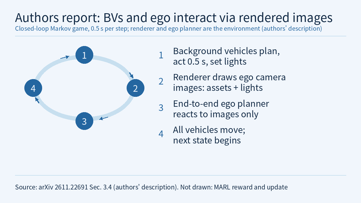
The authors then write the closed loop as a Markov game: background vehicles are agents sharing one policy, and the renderer and the ego planner belong to the environment. At each 0.5 s step, every background vehicle plans a trajectory, executes its first 0.5 s and sets its signal-light states; the ego sees only images rendered with the enhanced assets and lights and responds; then all vehicles move to the next state by their actions. The imitation-learned policy is frozen, and only a residual head is trained; it samples an offset on the displacements from a Gaussian whose mean is initialized to zero.
The reward works at the level of distributions. For each interaction phase, the onset to the end of an acceleration or deceleration, three features are extracted: TTC at onset, the signed peak acceleration a_max during the phase and the relative speed at its end. For each feature, the histogram count q on training logs is compared with the count p over the current iteration’s episodes, and the reward takes log(q/p), so values that are rarer in current rollouts than in the logs score higher; penalties for collisions, going off-road and progress deviation are subtracted. Optimization follows MAGRPO: each scene runs G episodes from the same initial state and ego seed, so episodes differ only in the sampled residuals, and all exploring background vehicles share the group-relative advantage of the team return. The objective is clipped, with a KL term that keeps the policy close to the initial one.
The evaluation uses the 288 long-tail navtest failure scenarios of NAVSIM, drawn from 89 nuPlan logs. Each episode runs 12 steps of 0.5 s with 8 surround cameras. The ego planner is Alpamayo 1.5, fed only the front camera at 2 Hz and never fine-tuned. All methods share the scenarios, ego planner, enhanced assets and light signaling and differ only in the component under evaluation. Background-vehicle policies are fine-tuned on nuPlan navtrain scenarios, which share no logs with the test set. Interaction realism compares the three feature distributions of closed-loop rollouts with the logs over 1,715 dynamic background vehicles, using Jensen–Shannon (JS) divergence and histogram overlap, alongside the background-vehicle collision rate and route progress.
The table below is taken from Table 1 of the paper (reported by the authors). RealEngine’s background vehicles are driven by DiffusionDrive planners and run in the authors’ own loop and renderer; OmniNWM’s background-vehicle states are estimated from generated videos; the “collisions” in the log reference row are overlaps of logged boxes.
| Method | TTC overlap ↑ | a_max overlap ↑ | Relative-speed overlap ↑ | Mean overlap ↑ | Mean JS ↓ | Collision rate ↓ | Progress (m) ↑ |
|---|---|---|---|---|---|---|---|
| Log reference | – | – | – | – | – | 3.50% | 27.66 |
| RealEngine | 0.8588 | 0.4324 | 0.6778 | 0.6563 | 0.1152 | 12.71% | 20.30 |
| OmniNWM | 0.7455 | 0.1492 | 0.8544 | 0.5830 | 0.1886 | 23.08% | 14.65 |
| World Engine | 0.9527 | 0.5771 | 0.8498 | 0.7932 | 0.0485 | 10.38% | 25.91 |
| Authors’ method | 0.9775 | 0.8719 | 0.9102 | 0.9198 | 0.0074 | 9.74% | 28.10 |
Mean JS divergence falls from World Engine’s 0.0485 to 0.0074, the 85% reduction the authors cite. Their reading is that for every compared method a_max is the worst-matched feature (overlap at most 0.58), while TTC is matched far better (up to 0.95): background vehicles start reacting at about the right time but react in the wrong way. The errors go in opposite directions. World Engine’s background vehicles react about twice as hard as the logged vehicles (median |a_max| of 4.7 vs. 2.3 m/s²); RealEngine’s decelerate in 73% of interaction phases, against 46% in the logs, and travel 27% less. The authors’ method keeps route progress within 2% of the logs. In the ablation, deploying the imitation-learned policy without closed-loop fine-tuning raises mean JS divergence by 77% (paired difference +0.0057, 95% CI [+0.0021, +0.0092]). Facing an ego that plans from rendered images, those background vehicles over-brake: they decelerate in 66% of interaction phases and travel 9% less. Closed-loop fine-tuning lowers the decelerating share to 50%.
Vehicle appearance: repairing only what interactions expose and the log does not constrain
A vehicle in a log is filmed from only a few directions. The authors diagnose each Gaussian of a vehicle asset individually: from the camera azimuth relative to the Gaussian and its blending weight in each training view, they accumulate its observational support at each azimuth. The left–right mirrored copy that MTGS keeps for each Gaussian also counts toward support, at a discount. The asset is then rendered from probe views, which combine uniform 360° views with higher-weighted interaction-critical views taken from ego-camera directions in closed-loop rollouts (for example, during a cut-in). A Gaussian’s “deficiency” is the share of its contribution that lacks observational support, so Gaussians that interactions expose but the log does not constrain score high.
Repairs come in two kinds. A native Gaussian with high deficiency shows colors extrapolated from unsupported directions, so the authors scale its view-dependent spherical-harmonic coefficients by (1 − deficiency) and keep its base color. Never-observed surfaces contain no Gaussians at all and are invisible to the deficiency score; these holes are filled from a donor asset. Asset Harvester generates the donor by multi-view synthesis from the vehicle’s image crops in the log, and only donor Gaussians whose share of contribution on pixels left empty by the native asset exceeds a threshold u0 are added. The repaired asset is fine-tuned on training images and finally processed in image space in two steps: a per-camera, per-channel color calibration, then a lightweight U-Net that decides per pixel how much of a diffusion harmonizer’s (DiffusionHarmonizer) correction and how much of a donor residual to accept, plus a free residual whose magnitude is bounded.
Simulated interactions have no ground truth, so the authors hold out all camera images and LiDAR at selected timestamps of 11 nuPlan logs and render the full scenes at the real camera and vehicle poses, evaluating 1,184 held-out images and 365 vehicle regions. All methods share the MTGS background and differ only in the target vehicle assets or post-processing. The table below is from Table 2 of the paper (reported by the authors):
| Method | Vehicle PSNR ↑ | Vehicle SSIM ↑ | Vehicle LPIPS ↓ | Full-image PSNR ↑ |
|---|---|---|---|---|
| MTGS | 17.05 | 0.411 | 0.466 | 18.17 |
| Difix3D+ | 16.91 | 0.396 | 0.415 | 18.18 |
| DiffusionHarmonizer | 17.11 | 0.406 | 0.432 | 18.08 |
| Asset Harvester | 15.24 | 0.359 | 0.504 | 18.06 |
| World Engine | 15.97 | 0.375 | 0.490 | 18.08 |
| Authors’ method | 17.97 | 0.438 | 0.448 | 19.01 |
The authors’ method scores a vehicle-region PSNR 2.0 dB above World Engine. The two methods that replace whole vehicles with generated assets (Asset Harvester and World Engine) fall 1.1–1.8 dB below the unenhanced MTGS reconstruction; the authors explain that a generated asset looks plausible but overwrites regions observed in the log with content that no longer belongs to that vehicle. The whole-frame diffusion enhancers (Difix3D+ and DiffusionHarmonizer) reach lower LPIPS by sharpening textures, with Difix3D+ the lowest, but vehicle SSIM drops and PSNR barely changes. The authors’ LPIPS is not the best, which they describe as a deliberate preference for fidelity to the logged vehicle over sharpness. In the ablation, diagnosis-guided repair is the largest single step, contributing 0.54 dB, nearly 60% of the total gain.
Signal lights: counterfactual fine-tuning for light states the log never showed
Each background vehicle’s light states follow its own plan and intention. The brake light turns on when the planned deceleration exceeds a threshold; with a lane-change intention, the turn signal on that side turns on before the visible lateral motion and blinks with a 1 s period until the lane change finishes. To keep lamp positions stable across frames, the authors anchor lamps in 3D on each asset: lamp masks segmented in the log images are back-projected into the vehicle’s box frame using the rendered depth, only voxels hit from multiple views are kept, and unseen sides are mirrored left to right.
The difficulty is that a log shows each vehicle only under the intentions that actually occurred, and so in few light states; how a vehicle would look braking instead of cruising has no paired image. The authors fine-tune the one-step diffusion model Difix with LoRA into an editor. Its inputs are the rendered vehicle crop, a reference view of the same vehicle with its observed light state, the lamp map and a state map marking the lamps to be lit; its output is composited only inside the lamp mask. During training the light state is flipped while all other inputs stay fixed. The output under the observed state is compared with the real photo through reconstruction losses (L1 and LPIPS); the flipped output must make a frozen ResNet-18 light-state classifier read the flipped state, and a further term penalizes hue drift of lit lamps.
Light-state correctness is read out by an independent vision-language model, Qwen2.5-VL-7B, never used in training. The brake-light evaluation covers 435 bidirectional counterfactual edits (115 vehicles); the turn-signal evaluation covers 272 left/right activations (136 vehicles). The authors’ method reaches a brake-light macro-F1 of 0.839 (FLUX: 0.830) and a turn-signal macro-F1 of 0.769 (FLUX: 0.685). General editors repaint 4%–88% of the body pixels, while the authors’ method changes less than 0.2% (0.14% and 0.06% with same-state and target-state photo references). For every editor, switching a light off is harder than switching it on, and deactivation is also the authors’ main failure mode. In the ablation, removing the counterfactual loss drops on-recall for vehicles observed only with lights off from 86.1% to 35.4%; the authors state that the 3D anchors do not improve single-frame accuracy (without them the brake-light mF1 is 0.845, against 0.839 for the full method) and are used for temporal stability: removing them raises the lamp-center jump rate by 9.5 points (95% CI [+5.0, +14.3]).
To test the effect of the lights on the ego, the authors run the 288 scenarios with and without light rendering under otherwise identical settings. The ego trajectory deviates by more than 10 cm in 24.3% of the scenarios for Alpamayo 1.5 and in 21.5% for openpilot. For Alpamayo 1.5, the lights change the planner’s front-view input images in 36% of the scenarios, and the trajectory deviates in 67% of those, by 0.77 m on average. From this the authors conclude that a world model with static lights changes the tested ego behavior in about a quarter of long-tail scenarios.
Limitations
- This is an arXiv preprint; all numbers are reported by the authors and have not been independently reproduced. The text read for this article gives no code or data link.
- The compared methods do not run under identical conditions: RealEngine’s background vehicles run in the authors’ own loop and renderer, and OmniNWM’s background-vehicle states are estimated from generated videos. The paper states that confidence intervals come from scene- or vehicle-level paired bootstrap, but the text read gives intervals only for some ablations; the values in Tables 1 and 2 carry none.
- The behavior reward targets the same three interaction-feature distributions used in the evaluation, although the reward uses training logs that share no logs with the test set. Being “closer to the logs” is therefore partly the optimization target itself; this is this site’s inference, not a statement in the paper. Distribution matching is also not a safety validation: the background-vehicle collision rate of the authors’ method, 9.74%, is still above the 3.50% of the log reference (where a “collision” is an overlap of logged boxes).
- Each episode is 12 steps of 0.5 s, or 6 s, and the ego planner uses only the front camera. The effect of lights on the ego was measured for two planners only, Alpamayo 1.5 and openpilot, with a 10 cm deviation threshold.
- Light-state correctness is read out by a vision-language model, not by human annotation. Novel-view fidelity is measured on held-out real frames; the novel views produced by interactions have no ground truth.
Links
- Making the World React Realistically: A Closed-Loop Interactive World Model for Autonomous Driving (arXiv 2611.22691)
- Full paper in HTML
- Physical AI Lab 3.2: World Models — Making Data with Cosmos, Writing Down What Each Kind of Generation Is Conditioned On, Putting 78.3% Back in Its Human Evaluation, Then Setting Acceptance Rules for Generated Data
- Frontier Radar | WorldFailBench: when a world model evaluates a policy, check failure reason, stage and boundary, not just success rate
- Physical AI Lab: a physical AI course where every number can be checked