The preprint CucumberVision at the Edge (arXiv 2611.09490, 2026-11-06, Kaur et al., University of Windsor and MBZUAI) moves an RGB-D cucumber length-measurement pipeline from a laptop with an RTX 3050 Ti to an NVIDIA Jetson Orin Nano and a Raspberry Pi 4, and reports length error, time per fruit and energy per fruit together. For anyone deploying vision at the edge, the paper gives three results to check against their own work: measurement accuracy is set by the segmentation backend, and for prompted backends at FP32 it differs by no more than 0.01 cm between the laptop and the embedded boards; after whole-graph INT8 quantization the detector returns no objects at all, because of how its output tensor is laid out; and the Jetson’s 7 W mode uses 73% more energy per fruit than its 15 W mode. All numbers below are reported by the authors [R]; this site has not reproduced them.
Setup: three machines replaying the same captures
The pipeline is the one from the authors’ earlier work (arXiv 2606.22439). An Intel RealSense D435 provides aligned colour and depth, a YOLO26n instance-segmentation model locates each cucumber, a segmentation backend refines the detection box into a pixel-level mask, and a medial arc spline estimator (M5 in the paper) fits a cubic spline through the cross-section centroids of the masked point cloud and integrates its arc length. In the paper’s schematic of an idealised curved fruit, the chord measured along a straight principal axis is 13% shorter than the arc, and the gap grows with curvature. Two other estimators, M1 and M2, use only the detection box, and the authors treat them as a control on the detector: if a change moves M1 and M2, it changed the boxes; if M1 and M2 stay put while M3 and M5 move, it acted through the segmentation stage.
- Laptop: RTX 3050 Ti, PyTorch CUDA, FP32, active cooling; the accuracy baseline.
- Jetson Orin Nano: JetPack 6.0, TensorRT 8.6.2, FP32 and FP16, active cooling.
- Raspberry Pi 4 B: Cortex-A72 CPU, 64-bit RPi OS, ONNX Runtime, FP32 and INT8, passive cooling.
All three machines replay the same 50 greenhouse captures, taken in two sessions as repeated views of 7 cucumbers, with thread-measured ground-truth lengths of 6.9–25.0 cm. Latency is computed over 220 post-warm-up captures and accuracy over all 50. YOLO26 needs no NMS and emits a tensor of shape (1, 300, 38); both boards skip the general-purpose inference wrapper and parse that tensor directly (except for configurations marked † in the tables).
The statistics are worth noting. Repeated captures of the same cucumber are not independent samples, so every interval in the paper uses a cluster bootstrap that resamples fruit (10,000 replicates), paired comparisons use an exact sign-flip permutation test in which all captures of a fruit change sign together, and the significance discussion gives the sample size as “7 specimens”. Physical AI Lab 2.8 sizes an evaluation from 1/√n on the assumption that runs are independent; this paper is a counterexample, where 50 captures are not 50 independent samples.
Under this protocol, the laptop and the Jetson at FP32 with SAM ViT-B both reach an M5 MAE of 0.58 cm (95% CI 0.46–0.69), with a Bland–Altman bias of +0.06 cm and a paired difference of zero. TensorRT FP16 cuts the Jetson’s detection latency from 120 ms to 46 ms (2.57×) and moves M5 to 0.64 cm; the paired difference is +0.061 cm (95% CI +0.005 to +0.137, p = 0.11), which the authors describe as consistently signed but not significant at 7 specimens. Building the FP16 engine warned that 115 weights fell outside the FP16 representable range; the authors checked and found the outputs within 1 px of the FP32 path in box coordinates and within 0.001 in confidence.
Accuracy follows the segmentation backend, cost follows the platform
Changing only the segmentation backend on one GPU gives 0.58 cm for SAM ViT-B, 0.76 cm for the distilled MobileSAM (95% CI 0.56–1.00) and 0.98 cm for the detector’s own YOLO-seg masks (95% CI 0.66–1.24). Across platforms, with FP32 on both sides, the two prompted backends (SAM and MobileSAM) differ by at most 0.01 cm between the laptop and the embedded boards. The masks themselves are almost pixel-identical: SAM’s mask IoU on the Jetson at FP32 is 1.000, and MobileSAM on the Raspberry Pi matches the laptop at a mean IoU of 1.000 (minimum 0.997).
Cost does not transfer across platforms at all. MobileSAM takes 70 ms on the laptop and 15,041 ms on the Raspberry Pi, a factor of 214. From this the authors argue that backend selection and platform selection can be made separately: evaluate candidate backends on a workstation in minutes, treat the resulting accuracy as what the field system will deliver, then pick the platform for throughput and energy. They state three boundary conditions:
- It holds only for prompted backends. With the detector’s own masks, M5 is 0.98, 0.82 and 0.84 cm on the laptop, Raspberry Pi and Jetson, mask IoU between the Raspberry Pi and the laptop averages 0.823 with a minimum of 0.447, and on both embedded boards native-mask configurations show a systematic bias of about +0.57 cm, a tendency to overestimate length.
- The backends compared are deterministic given the same prompt.
- Mask quality has to clear a threshold. The classical GrabCut costs 2.4× less than MobileSAM but fails to produce a usable mask on 22% of frames, and M5 degrades to 1.92 cm, worse than M2 (0.83 cm), which needs no mask at all.
Whole-graph INT8: the fastest detector on the Raspberry Pi, and it finds no fruit
In the detector quantization ablation on the Raspberry Pi, the calibration data were 40 held-out greenhouse frames. The authors exported the detector to ONNX and applied static post-training quantization in QDQ format, comparing four strategies: per-tensor MinMax, per-tensor entropy, per-tensor percentile and per-channel MinMax. Quantizing the whole graph shrinks the model from 41.7 MB to 11.1 MB, cuts peak memory from 682 MB to 460 MB and reduces detection latency from 1,929 ms to 793 ms (2.43×), the fastest detector measured on the Raspberry Pi in the study. It also returns no detections on any capture, on two platforms and two ONNX Runtime versions.
The authors trace the cause to the output layout. The NMS-free detection head emits a single tensor whose box coordinates span 0–640 and whose confidences span 0–1. Per-tensor quantization gives the whole tensor one scale, which the coordinates have to set; the paper gives the resulting step as 7.71. A peak confidence of 0.85 is 0.11 of one step and rounds to zero, so no candidate box clears the detection threshold. The authors’ argument: keeping 0.85 non-zero requires a step below 1.63, while representing 640 in 255 unsigned levels requires a step of at least 2.51. The two requirements exclude each other, so no calibration strategy can avoid the failure, and changing weight granularity does not help either. On this basis the paper attributes the failure to the output layout, not to this model, dataset or toolchain; the precondition is that coordinate-scale and probability-scale values share one tensor that is quantized per tensor.
The fix is to leave the detection head out of quantization (it holds 12.6% of the convolution weights). The model is then 15.1 MB, peak memory 594 MB and detection latency 1,406 ms, a 1.37× speed-up; M5 moves from 0.82 cm to 1.12 cm (+0.30 cm, 95% CI −0.03 to +0.83, p = 0.27), and the Bland–Altman limits of agreement widen to −3.43 to +3.69 cm.
Physical AI Lab 2.6 keeps weight size, runtime memory and latency as three separate accounts when assessing quantization. This case adds a check that comes before all three: whether the output is still valid. Whole-graph INT8 is best on size, memory and latency, and detects nothing; a choice made from the speed table alone would be wrong. The measurements collected in the edge and real-time deep dive showed quantization saving memory and running slower; here, with the head excluded, detection on the Raspberry Pi’s CPU does get 1.37× faster, at a cost of 0.30 cm more error (an interval that includes zero).
Energy per fruit: lower power does not mean less energy
On the Jetson, the on-board INA3221 monitors (read through tegrastats) give the VDD_IN rail power, which is integrated over the active window and divided by the number of fruit measured; an idle baseline is recorded for each power mode and subtracted to give a net figure. The Raspberry Pi has no on-board power sensor, so the authors measured its supply power externally, against an idle baseline of 2.52 W. Each run measures 44 fruit (Table 5 of the paper):
| Configuration | Mean draw (W) | Run time (s) | J/fruit | J/fruit (net) | M5 MAE (cm) |
|---|---|---|---|---|---|
| Jetson TensorRT FP16 + SAM, 15 W | 10.14 | 183 | 42.18 | 20.18 | 0.64 |
| Jetson TensorRT FP16 + SAM, 7 W | 7.21 | 446 | 73.12 | 23.45 | 0.64 |
| RPi 4 FP32 + MobileSAM | 5.41 | 859 | 105.55 | 56.38 | 0.76 |
| RPi 4 FP32, native masks | 5.68 | 117 | 15.05 | 8.38 | 0.82 |
| RPi 4 INT8 (head FP32), native masks | 5.61 | 89 | 11.29 | 6.22 | 1.12 |
The 7 W mode draws 29% less power but takes 2.44× as long, so each fruit costs 73.12 J, 73% more than the 42.18 J of the 15 W mode. Accuracy is bit-identical in the two modes (M5 is 0.64 cm in each, with a paired difference of exactly zero), which the authors use as a control: a power cap changes execution speed, not arithmetic. Most of the slowdown is in the segmentation stage, which slows by 2.75× against 1.49× for detection. From the net figures in the table, this site calculates the gap at about 16% (23.45 against 20.18 J), so most of the 73% gross gap is idle power accumulated over the longer run. The gross figure is what the battery actually pays; from the 15 W mode’s gross figure of 42.2 J per fruit, the authors estimate that a 100 Wh battery supports about 8,500 measurements.
The same accounting holds between platforms. The Raspberry Pi running MobileSAM draws 5.41 W, 47% less than the Jetson’s 10.14 W with SAM, yet uses 105.55 J per fruit, 2.50× the Jetson’s gross figure and 2.79× its net figure, and these are the two configurations closest in accuracy (0.76 against 0.64 cm). Load power on the Raspberry Pi is nearly constant across configurations (5.41 to 5.68 W, a 5% spread), so any latency reduction there saves energy in the same proportion: INT8 with the head excluded cuts energy per fruit from 15.05 J to 11.29 J, 25% less. The Jetson does not behave this way, because its power mode changes both the draw and the duration. The EdgeVLN article on this site likewise compares execution paths by energy per step rather than by power.
On thermals, the passively cooled Raspberry Pi ran the quantized pipeline continuously for 30 min (21 °C laboratory ambient), reached thermal equilibrium in about 90 s and peaked at 53.0 °C, 27.0 °C below the 80 °C throttle threshold. The ARM clock held 1800 MHz across all 357 samples, no throttle flag was set, and per-run detection latency varied by 1.1%.
Three non-dominated configurations and rules for choosing
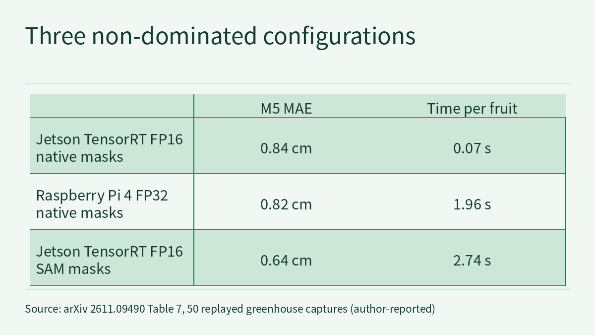
Table 7 of the paper places each configuration in accuracy–throughput–energy space, judges dominance on accuracy and throughput, and, among the embedded deployment configurations (the laptop reference row is excluded), marks three as non-dominated:
- Jetson TensorRT FP16, native masks: M5 0.84 cm, 0.07 s (72 ms) per fruit, about 0.7 J per fruit (derived).
- Raspberry Pi 4 FP32, native masks: 0.82 cm, 1.96 s, 15.1 J per fruit; the low-cost option.
- Jetson TensorRT FP16, SAM: 0.64 cm, 2.74 s, 42.2 J per fruit.
Between the two operating points on the same Jetson, a 38× latency difference buys 0.20 cm of accuracy. The authors draw three rules from the ablations, which can be applied together: choose the segmentation backend for the accuracy target, evaluated on whatever hardware is convenient, since the accuracy of prompted backends transfers; choose the platform for the throughput and energy target, since the platform does not change the accuracy the backend delivers; and quantize the detector only where it is the bottleneck (on this pipeline, the native-mask configurations), excluding the detection head.
Two things are worth keeping in mind when reading the table; this is this site’s reading. The Raspberry Pi native-mask configuration is “non-dominated” because of a 0.02 cm gap, 0.82 against 0.84 cm, while the two 95% CIs (0.66–0.98 and 0.69–0.98) almost coincide. The authors also state that dominance counts only accuracy and throughput, not hardware cost, so a dominated configuration may still be the right choice on cost. And the roughly 0.7 J for the Jetson native-mask configuration is derived from per-fruit latency and mean draw, not measured.
Limitations
- This is an arXiv preprint; all numbers are reported by the authors [R] and have not been reproduced by this site. According to the paper, the code, quantization configurations, energy and thermal harnesses and result files are available from the corresponding author on request; there is no public repository.
- The sample is small: replays of 50 stored captures of 7 cucumbers, all single-fruit frames. The paper also mentions in-lab real-time length estimation with the RGB-D camera mounted on the robot end, but the result tables this site read all come from the replays.
- One unit of each board was tested, so unit-to-unit variation is not characterised; the thermal test was run once at 21 °C laboratory ambient, and extending it to greenhouse ambient is a single-condition inference, as the authors also state.
- The paper reports no mAP, because there are no independently annotated ground-truth boxes; two energy entries in Table 7 are derived from latency and mean draw.
- While checking, this site noticed that the Table 5 run time divided by 44 fruit is longer than the per-fruit latency in Table 2 (for example, 183 s / 44 ≈ 4.2 s for the Jetson SAM configuration, against 2.74 s in Table 2). The text this site read does not explain the difference, so J/fruit should not be back-calculated from Table 2 latencies.
- The INT8 failure argument applies to the precondition of coordinates and confidences in one tensor quantized per tensor; other output layouts or quantization schemes are outside the paper’s conclusions.
- All results are measurement-accuracy and compute-performance figures; none of them is a safety validation of robot motion.
Links
- CucumberVision at the Edge: Accuracy, Throughput, and Energy of RGB-D Cucumber Sizing on Jetson Orin Nano and Raspberry Pi 4 (arXiv 2611.09490)
- Full paper in HTML
- Physical AI Lab 2.6: To the Edge — Working Out the Control-Rate Ceiling from a Latency Log, Telling Whether Quantization Saves Size or Time, Then Sizing an Action Chunk
- Physical AI Lab 2.8: Reproducible Evaluation — Working Out Wald and Wilson Intervals by Hand, Sizing a Run from 1/√n, Then Bounding the Failure Rate after Zero Failures
- Frontier Radar deep dive | Edge and real-time: where the latency budget of VLAs and world action models goes
- Frontier Radar | EdgeVLN: same 4 bits, 36.8× difference in step energy depending on the execution path