A preprint from authors at the University of Genoa’s DITEN department and others (arXiv 2611.07779, 2026-11-05) seals two flexible piezoelectric tactile arrays in silicone to make two removable “sensing caps”. The caps fit over both sides of a TIAGo robot’s gripper and carry 32 sensing points in total; the goal is to recognize the grasped object at the very start of the grasp. The authors report that with all 32 sensing points and a window of 50 samples at 500 Hz (100 ms), turning the signals into spatio-temporal heatmaps for a 2D-CNN gives an F1-score of 0.9903 on six everyday objects. Deployed on an STM32 microcontroller, the model has an end-to-end latency of about 101 ms from contact onset and uses 63.8 µJ per inference. Two points make the paper worth a close read. Piezoelectric signals respond only to change, which matches the moment of first contact. And nearly 100 ms of the 101 ms is spent waiting for the data window to fill, not computing. All numbers below are reported by the authors [R]; this site has not reproduced them.
The system: two sensing caps, 32 points, 500 Hz
JOANNEUM RESEARCH screen-printed each sensor array. Bottom electrodes are printed on a 100 µm flexible PCB, followed by a 5.1 µm layer of the ferroelectric polymer P(VDF-TrFE) and PEDOT:PSS top electrodes; a UV-cured lacquer protects the stack, and the layer is poled through its thickness. One array is a 4 × 4 grid of 16 sensing points with 5 mm spatial resolution. The authors cast an inner silicone cap shaped to the gripper in a 3D-printed mould, glued the array onto it and poured a second silicone layer; the array is packaged in the skin-like compliant material Dragon Skin. This gives two sensing caps, SC1 and SC2.
The readout reuses the group’s earlier embedded electronics: a 32-channel analog-to-digital converter (DDC232) and a low-power Arm Cortex-M0 microcontroller sample all 32 channels at 500 Hz and send them over a flat cable to a host PC, where a LabVIEW interface records them.
The sensor characterization is taken from the group’s earlier paper: sensitivity rises with frequency, from 1.5 to 31.96 pC/N; nonlinearity error is 2.3%; SINAD is about 56 dB. This paper adds tests with an electromechanical shaker and a rigid 4 mm indenter. Under 1–100 Hz sine stimulation the output voltage rises with frequency to a maximum of about 5 mV, which the authors attribute to the shaker’s transfer function (its indentation force itself depends on frequency). Under square stimuli from 0.12 to 6 N the output is roughly linear in force.
Why piezoelectric sensing suits the moment of contact
A piezoelectric material produces charge only while the force on it changes. Fig. 4 of the paper records TIAGo picking up the half-filled bottle. When the gripper closes, all 32 signals rise quickly; in the hold phase the force becomes quasi-static and the signals fall back, leaving only small wiggles from gripper vibration or the bottle deforming; on release there is another peak. The authors conclude that piezoelectric sensors suit dynamic forces during motion, such as judging object properties at the first instant of touch, rather than static grip force.
The experiment uses six objects: a glass bottle, a TV remote, a half-filled plastic water bottle, and three 3D-printed fruits from the YCB object set (strawberry, rigid apple, semi-soft apple). The robot runs a fixed approach–grasp–hold–release sequence, 50 times per object, for 300 trials in total; the object’s position and orientation in the gripper change between trials.
Three recognition routes, and how the data were split
Each trial’s signal is cut into windows of length W, with W set to 50, 100, 150 or 200 samples. The authors compare three routes:
- Feature-based (FBA): 8 statistical features are computed per sensing point per window; ranking them with a PCA biplot keeps 4 (energy, peak-to-peak, maximum, minimum), which go to an SVM with an RBF kernel.
- Raw signal (EEA): normalized raw waveforms go straight into a 1D-CNN or a C-RNN (convolutional layers followed by an LSTM).
- Heatmap (HMA): within each window, the absolute maximum of each sensing point is taken and min–max normalized per point, then laid out as two small matrices following the physical arrangement on the two caps (two 4 × 4 matrices for 32 points). These go to a 2D-CNN with a single convolutional layer (32 kernels of 2 × 2).
The number of sensing points is chosen by activity: each point’s normalized energy is computed, the median over the 300 trials ranks them, and the most active 4, 8, 16 and 24 points, plus all 32, form the groups. In the PCA plots the silhouette score is 0.08 with 4 points and 0.16 with 16; between 16, 24 and 32 points it differs only on the order of 10⁻³. The authors therefore carried only the 16-, 24- and 32-point groups into the recognition experiments.
The data split is one of the clearer parts of the paper. The authors note that cutting windows before splitting into training and test sets lets highly correlated segments from the same grasp land in different subsets, which leaks information. They split by whole trials first: taking the class with the fewest samples as reference, 70% of each class goes to training and the rest is divided 15% and 15% between validation and test; only then are windows cut inside each subset, so every window from one grasp stays in one subset. The paper does not state how many trials are in the test set; if the unit of the split is the trial, 15% of 50 trials per class is about 7–8 trials (this site’s estimate).
Results: more sensing points help, shorter windows help
The table gives F1-scores at W = 50 (Table V and the text of the paper; the two EEA models are listed separately):
| Route and model | 16 sensing points | 24 sensing points | 32 sensing points |
|---|---|---|---|
| HMA: heatmap + 2D-CNN | 0.9796 | 0.9846 | 0.9903 |
| FBA: features + SVM | 0.9445 | 0.9604 | 0.9661 |
| EEA: raw signal + 1D-CNN | 0.9006 | 0.9385 | 0.9618 |
| EEA: raw signal + C-RNN | 0.8824 | 0.9102 | 0.9532 |
Two things stand out. First, the silhouette scores suggest that going beyond 16 points barely helps clustering, yet the F1 of all four models still rises with more points; the authors attribute this to random grasp positions activating different points in different trials. Second, the heatmap route with only 16 points (0.9796) already beats the best results of the other two routes with all 32 points (0.9661 and 0.9618). One sentence in the paper says the heatmap route reached 0.9846 “even when trained on half of the sensors”, but in Table V 0.9846 belongs to 24 points and 16 points give 0.9796; the conclusion holds under either reading.
The window-length trend runs against intuition: longer windows lower the F1 of every route. With 16 points, the 2D-CNN falls from 0.9796 at W = 50 to 0.9077 at W = 200, and the SVM from 0.9445 to 0.9253; the 1D-CNN and C-RNN fall most, by about 11% as the paper puts it; with 32 points, the paper describes the drop for the 2D-CNN and SVM as about 2%. At 500 Hz, W = 200 corresponds to 400 ms (this site’s conversion). The authors explain the trend by the sensors’ high bandwidth and fast response, so a short window already holds enough spatio-temporal information. One factor the paper does not discuss separately: the number of windows per trial is the sample count divided by W, so a larger W leaves fewer windows for training (this site’s inference).
Where the 101 ms goes
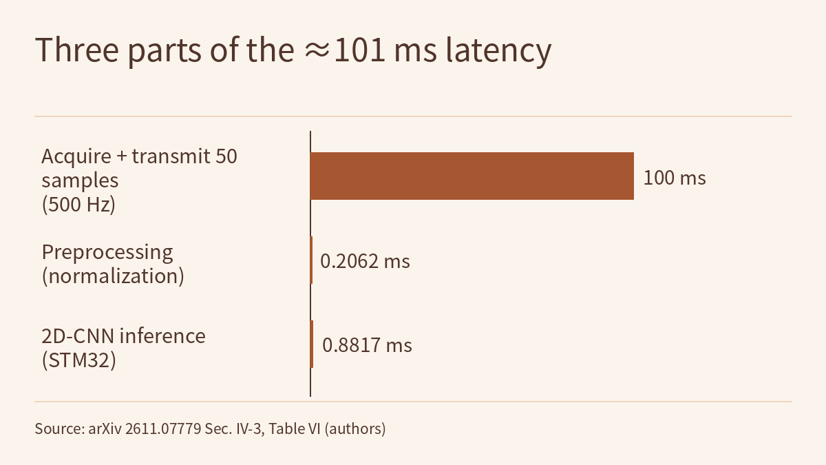
The authors deployed the 32-point, W = 50 2D-CNN on an STM32 microcontroller with an Arm Cortex-M4F core (using STM32CubeIDE) and report these hardware figures: inference time 0.8817 ms, power 72.3 mW, energy 63.8 µJ per inference, 7.65 kB of flash and 11.3 kFLOPs per inference. 72.3 mW times 0.8817 ms is about 63.7 µJ, in line with the reported value (this site’s check).
The end-to-end latency is the sum of three parts: acquiring and transmitting 50 samples at 500 Hz takes 100 ms, the on-board preprocessing (normalization) measured 0.2062 ms, and model inference 0.8817 ms, for 101.0879 ms in total. Computation takes about 1.1 ms; everything else is waiting for the window to fill. Recognizing earlier would mean changing the sampling rate or the window length, and the “shorter W, higher F1” trend was only measured between 50 and 200 samples; the paper tested no window shorter than 50. Citing earlier work, the authors say perception and grasp-planning pipelines that finish within about 100 ms are suitable for real-time manipulation, and use this to argue 101 ms is acceptable. That is the authors’ argument; the paper reports no closed-loop experiment in which the recognition result drives the robot’s manipulation.
Table I of the paper sets this work beside seven earlier studies of tactile object recognition and notes that none reports hardware deployment, and only one reports a response time, 103 ms on a GPU. Those studies differ in sensors, objects and tasks, so Table I is a feature comparison, not a performance comparison under equal conditions.
How this relates to the course on this site
Physical AI Lab 1.3 sorts sensors into cameras, depth, force and touch, and proprioception; its touch example is the kind that hides a camera behind a gel pad and watches the imprint. This paper shows a different kind of touch. A piezoelectric array outputs changes in charge: there is almost no signal while an object is held still, and peaks only at contact and release. It can therefore answer “what did I just touch?” but not “how tightly am I holding it now?”. In Frontier Radar’s report on PhysCanvas, touch enters a world model as images and marker displacements, which makes a useful contrast in what tactile data look like.
Physical AI Lab 2.6 practises splitting a latency log into its stages. The 101 ms here is a ready-made example: once waiting for data is separated from computing, it is clear that a faster chip would barely shorten this latency.
Limitations
- This is an arXiv preprint; all numbers are reported by the authors [R], and this site has not reproduced them. The text this site read gives no code or dataset address.
- Limitations stated by the authors: a small object set (6 objects), a single robot platform and one predefined grasp–hold–release interaction. The three fruits are 3D-printed, not real fruit.
- The paper does not state the number of test trials or windows, and reports no variance or confidence intervals over repeated training runs. The differences between 0.9796, 0.9846 and 0.9903 may correspond to only a few windows; this site cannot judge whether they are stable.
- Judging from the paper’s dataset definition (each whole trial is cut into windows of length W), this site reads F1 as computed over all windows cut from the whole grasp sequence, including the hold and release phases; the paper does not say which windows the test F1 includes. The text this site read does not report recognition on “the first window after contact” separately, nor explain how contact onset is detected online. “Recognizing the object from the first 50 samples after contact” is the authors’ conclusion; the numbers in the tables do not measure it directly.
- The 101 ms is a sum of three parts: the paper counts acquiring and transmitting 50 samples at 500 Hz together as the 100 ms window time, while preprocessing and inference were measured on the STM32. The text does not itemize the transmission time within it, and reports no closed-loop result in which the recognition drives the robot’s manipulation.
- 63.8 µJ is the energy of one model inference only; it excludes the sensors, the analog-to-digital converter and the acquisition board.
- The abstract says tactile sensing often outperforms vision-based solutions in enabling safe, efficient grasping, because it gives direct information about physical properties such as texture and shape, but this study has no vision baseline; that sentence is background, not an experimental result of the paper.
- Recognition accuracy is not a validation of grasp safety or reliability. The paper does not test slip, more objects or other grippers; the authors list these as future work.
Links
- Flexible Piezoelectric Tactile Sensing System for Intelligent Object Recognition (arXiv 2611.07779)
- Full paper in HTML
- Physical AI Lab 1.3: Sensors — Working Out Pixels, Depth Range and Grip Force for One Cup
- Physical AI Lab 2.6: To the Edge — Working Out the Control-Rate Ceiling from a Latency Log, Telling Whether Quantization Saves Size or Time, Then Sizing an Action Chunk
- Frontier Radar | PhysCanvas: drawing vision, touch and task state on one canvas, then using three frozen reward models to bring world-model outcomes closer to the real robot
- Physical AI Lab: a physical AI course where every number can be checked (course outline)